ZKP Notes
$$\newcommand{\bm}[1]{\boldsymbol{#1}}$$
Berkeley Workshop
The reason ZKPs are not a paradox is really because of timing. Well, timing and randomness. While it is true that a verifier could just spit out a transcript of a valid ZKP interaction, the prover is different in that it makes a commitment before the randomized challenge.
But you can turn an interactive proof into a non-interactive one with Fiat Shamir (make the challenge a hash of a commitment).
Interactive Proofs
- common trick
- extend functions to multilinear polynomials.
- rely on the fact that if polynomials are different, they differ in most places (strong statistically guarantees)
- arithmetic circuit
- encode boolean gates as arithmetic, forming an injection to a field
Probabilistically Checkable Proofs
- Verifier as efficient as possible
- Assume prover is computationally powerful
- Interaction not always feasible
- Ideas:
- What if the verifier selects random bits of the proof to verify?
- In this case, increase soundness by increasing # of bits to check
- What if the verifier selects random bits of the proof to verify?
Succinct Arguments
Motivation
Looking at arguments instead of proofs:
- why?
- they can be succinct
- proofs have computational limitations
- e.g. SAT prover/verifier requires $2^{\mathcal{O}(n)}$ in bits
- soundness is computational and applies to efficient provers
- interactive proofs (IP) are a subset of interactive arguments (IA)
Definition
- Define $R^\star$ to be a universal relation about all satisfiability problems together:
- $R^{\star} = { ((A, z, t), w) : A(z, w) \text{ in at most }t\text{ steps}}$
- $A$ is an algorithm,
- $z$ an input,
- $t$ a time bound
- $w$ a witness
- An interactive argument for $R^\star$ is succinct if
- communication complexity is small: $poly(\lambda, \log t)$
- verification time is small: $poly(\lambda, |A|, |z|, \log t)$
- verifier has to read the input!
- typically $t \sim poly(\lambda)$
Construction
We'll use a classical construction from 80s, to transform any PCP (Probabilistically Checkable Proof?) into a succinct argument:
- Theorem: $R^\star$ has good PCPs
- proof is not too big
- time to verify it is not too big
- communication is not too big
- First attempt:
- Verifier sends random $r$ to sample
- Prover restricts $\pi = P_{PCP}(A,z,t,w)$ to sample according to $r$
- Verifier verifies according to $V_{PCP}^{\pi'}(A,z,t,r)$
- This isn't correct! Prover shouldn't know $r$ ahead of time! Prover should commit to their proof ahead of time.
- Upgrade to:
- Prover has to commit to $\pi$ first via a merkle-tree built with a collision-resistant hash function.
- Verifier samples some hash function $h \leftarrow H_k$ (can't let prover choose it!).
- Prover builds a merkle tree $MT_h(\pi)$ of its proof, and sends the root $r_t$ of the tree.
- Then verifier sends random $r$.
- Prover deduces the query set $Q_r$ and computes paths for locations in $Q_r$.
- sends $(\pi|Q, paths)$ to verifier
- Verifier
- check paths w.r.t. $r_t, Q$
- decides according to $V_{PCP}^{\pi|Q}(A, z, t; r)$.
Non-interactive
When we want to make Succinct NonInteractive Arguments (SNARGs), instead of the verifier sending random $r$ to the prover, there is an initial Setup phase which outputs a Reference String. So lets remove the interactive bits above:
- Setup phase can choose the hash function $h \leftarrow H_k$ for the Merkle tree
- Setup phase can generate a hash $f \leftarrow F_k$ for a Fiat-Shamir transform
- Now the interactive $r$ is substituted with $f(r_t)$.
ZK Whiteboard Sessions
Module 1
A SNARK is just a way to prove a statement:
- Succinct Non-interactive Arguments of Knowledge
- basically a short proof (few KB) that is quick to verify (few ms)
A zk-SNARK is a SNARK but it doesn't reveal why the statement is true
Building blocks
- Arithmetic circuits: Given a finite field $\mathbb{F}$, a circuit $C: \mathbb{F}^n \to F$ defines an $n$-variate polynomial with an evaluation recipe in the form of a DAG, where inputs are labeled $1, x_1, \ldots, x_n$ and internal nodes are labeled $+, -, \times$.
- e.g. $C_{hash}(h, m) = 0$ iff $sha256(m) = h$.
- Argument system: Given public arithmetic circuit $C$, public statement $x \in \mathbb{F}^n$, and secret witness $w \in \mathbb{F}^m$, suppose we have two parties (V) verifier and (P) prover. An argument system consists of various messages passed between these parties, where P wants to convince V that there does exist $w$ such that $C(x, w) = 0$, but P only sends $x$, not $w$. Then V accepts or rejects P's argument.
- Non-interactive preprocessing argument system: An argument system augmented with a preprocessing step $S(C) \to (S_p, S_v)$ that produces public parameters. Then P has inputs $S_p, x, w$ and V has inputs $S_v, x$. P then sends a single proof message $\pi$ and V accepts or rejects it. This argument system is defined by the three algorithms:
- $S(C) \to (S_p, S_v)$.
- $P(S_p, x, w) \to \pi$.
- $V(S_v, x, \pi) \to {0, 1}$.
- We require:
- Completeness: if $C(x,w) = 0$, $V$ always accepts.
- Soundness: if $V$ accepts, then $P$ knows $w$; if $P$ does not know $w$, then probability of acceptance is negligible. (Note: this is not a logically sound definition. I assume the speaker intended the converse of the former.)
- Zero-Knowledge (optional): $(C, S_p, S_v, x, \pi)$ reveal nothing about $w$.
- Succinct Non-interactive preprocessing argument system: Further restriction that
- $P$ produces short proof: $|\pi| = O(\log(|C|), \lambda)$
- $V$ is fast: $time(V) = O(|x|, \log(|C|), \lambda)$
- Note: these $\log(|C|)$ requirements are exactly why we need a preprocessing step; otherwise the verifier would have to read the entire circuit to evaluate it.
- Arithmetic circuits: Given a finite field $\mathbb{F}$, a circuit $C: \mathbb{F}^n \to F$ defines an $n$-variate polynomial with an evaluation recipe in the form of a DAG, where inputs are labeled $1, x_1, \ldots, x_n$ and internal nodes are labeled $+, -, \times$.
Types of preprocessing steps:
- trusted setup per circuit: $S(C; r)$ where random $r$ must be kept secret from prover (otherwise it could prove false statements!)
- trusted but universal (updatable) setup: secret $r$ is independent of $C$:
- $S = (S_{init}, S_{index})$ where
- $S_{init}(\lambda; r) \to pp$ is a one-time trusted procedure to generate public params; afterwards throw away $r$
- $S_{index}(pp, C) \to (S_p, S_v)$ can then be used to deterministically preprocess any new circuits $C$ without any dangerous secret randomness
- transparent: S(C) does not use secret data, and there is no trusted setup. This is obviously preferrable.
- E.g.
- Groth'16: small proofs 200B, fast verifier time 3ms, but trusted setup per circuit
- Plonk/Marlin: small proofs 400B, fast verifier time, 6ms , but universal trusted setup
- Bulletproofs: larger proofs 1.5KB, verifier 1.5s, but no trusted setup.
A SNARK software system
- Typically a DSL is used to compile a circuit from a higher level language
- Then public params $S_p, S_v$ are generated from the circuit.
- Finally, a SNARK backend prover is fed $S_p, S_v$ and also $x, witness$ to generat a proof.
Some more formal definitions:
- The formal definition states that $(S, P, V)$ is knowledge sound for a circuit $C$ if:
- If an adversary can fool the verifier with non-negligible probability,
- then an efficient extractor $E$ which interacts with the adversary as an oracle, can extract $w$ with the same probability.
- (If $P$ knows $w$, then $w$ can be extracted from $P$.)
- $(S,P,V)$ is zero knowledge if
- there is an efficient algorithm $Sim$ such that
- $(S_p, S_v, \pi) \leftarrow Sim(C, x)$ looks like the real $S_p, S_v,$ and $\pi$.
- notice the simulator has more power than the prover - it can choose $S_p, S_v$!
- (If for every $x \in \mathbb{F}^n$, the proof $\pi$ reveals nothing about $w$ other than existence.)
- The formal definition states that $(S, P, V)$ is knowledge sound for a circuit $C$ if:
Module 2
zk-SNARK is generally constructed in two steps:
- A functional commitment scheme, and
- (cryptography happens here)
- A suitable interactive oracle proof (IOP)
- (information theoretic stuff happens here)
- A functional commitment scheme, and
A commitment scheme is essentially an "envelope". Commit to a value and hide it in the envelope.
- It consists of two algorithms
- $commit(m, r) \to com$
- $r$ is random
- $com$ is small even for large $m$, typically 32B
- $verify(m, com, r) \to \{0, 1\}$
- $commit(m, r) \to com$
- Satisfying properties:
- binding: cannot produce two valid openings for a single commitment $com$.
- hiding: the $com$ reveals nothing about the committed data (envelope is opaque!)
- Example: hash function
- $commit(m, r): com := Hash(m, r)$
- $verify(m, r): com == Hash(m, r)$
- It consists of two algorithms
We actually commit to a function $f \in \mathcal{F}$, where $\mathcal{F}$ is a family of $f: X \to Y$.
- Prover commits to $f$ and sends $com_f := commit(f, r)$ to verifier.
- Verifier sends $x \in X$
- Prover sends $y \in Y$ and proof $\pi$ which proves $f(x) = y$ and $f \in \mathcal{F}$.
A functional commitment scheme for $\mathcal{F}$:
- $setup(\lambda) \to pp$ outputs public params (one time setup)
- $commit(pp, f, r) \to com_f$
- SNARK requires binding
- zk requires hiding
- $eval(P, V)$ for given $com_f, x, y$:
- $P(pp, f, x, y, r) \to \pi$
- $V(pp, com_f, x, y, \pi) \to \{0, 1\}$
Examples
- KZG:
- where $f$ is a polynomial
- a trusted setup defines $pp$ around an $\alpha$ that is thrown out afterwards.
- commitments are simple algebraic operations around $\alpha$
- proofs are literally single elements from a group $\mathbb{G}$
- verifier is a constant time assertion of element equality using a tiny bit of public params.
- very elegant, aside from trusted setup.
- Dory:
- Removes trusted setup from KZG at the cost of:
- proof size $O(log d)$
- prover time $O(d)
- verify time $O(log d)
- Removes trusted setup from KZG at the cost of:
- KZG:
Module 3
Let $\omega \in \mathbb{F}_p$ be a primitive $k$-th root of unity. Set
$$H := {1, \omega, \ldots, \omega^{k-1}} \subset \mathbb{F}_p.$$
Let
$$ f \in \mathbb{F}_p^{(\le d)}[X] ; \text{ and } ; b,c \in \mathbb{F}_p \qquad (d \ge k) $$
- Gadgets: There are efficient poly-IOPs for:
- zero test: $f$ is identically zero on $H$.
- sum-check: $\sum_{a\in H} f(a) = b$
- product-check: $\prod_{a\in H} f(a) = b$
All of these are rather simple constructions relying on the fact that polynomials have highly unique outputs: consider the probability that a random $x$ is a root of $f$. Out of $p$ possible values for $x$, $f$ has at most $d$ roots, so the probability is $d/p$. If $p \approx 2^{256}$ and $d \le 2^{40}$, this is negligible.
PLONK poly-IOP for general circuit
- First, prover compiles a circuit to a computation trace. The computation trace is just a representation of the inputs at each of the gates.
- To encode as polynomial $P$,
- let $|C|$ be total # of gates in C,
- $|I| = |I_x| + |I_w|$ be the total # of inputs.
- $d = 3|C| + |I|$
- $H = {1, \omega, \ldots, \omega^{d-1}}$
- Encode gates as:
- $P(\omega^{3\ell})$: left input of gate $\ell$
- $P(\omega^{3\ell+1})$: right input of gate $\ell$
- $P(\omega^{3\ell+2})$: output of gate $\ell$
- To encode as polynomial $P$,
- Then, prover will prove
- $P$ encodes correct inputs
- every gate evaluated correctly
- wiring is implemented correctly (basically means equal values from one gate output get sent to the next gate correctly)
- output of last gate is zero: $P(\omega^{3|C|-1}) = 0$.
These steps are detailed below:
- To prove correct inputs:
- Both prover and verifier interpolate a polynomial $v(X) \in \mathbb{F}_p^{(\le |I_x|)}[X]$ that encodes the $x$ inputs to the circuit.
- $v(\omega^{-j}) =$ input # j.
- So all the points encoding the input are $H_{inp} = {w^{-1},\ldots,w^{-|I_x|}}$
- Hence prover can prove (1) with a zero test: $P(y) - v(y) = 0$ for all $y\in H_{inp}$.
- Both prover and verifier interpolate a polynomial $v(X) \in \mathbb{F}_p^{(\le |I_x|)}[X]$ that encodes the $x$ inputs to the circuit.
- To prove gates evaluated correctly, encode gates with a selector polynomial to pick out which ones are addition/multiplication:
- Define selector $S(X) \in \mathbb{F}_p^{(\le d)}[X]$ such that for all $\ell = 0, \ldots, |C| - 1$:
- $S(\omega^{3\ell}) = 1$ if gate #$\ell$ is an addition gate
- $S(\omega^{3\ell}) = 0$ if gate #$\ell$ is a multiplication gate
- Then for all gates $y \in {1, \omega^3, \omega^6, \ldots, \omega^{3(|C|-1)}}$:
- $S(y)[P(y) + P(\omega y)] + (1 - S(y))\cdot P(y) \cdot P(\omega y) = P(\omega^2 y)$.
- NOTE: selector only depends on circuit, not input, so it can be computed in the preprocessing step!
- So $Setup(C) \to S_p := S, S_v := (S')$ where $S'$ is a commitment to the selector polynomial $S$.
- Now proving happens via another zero-test on $S$ for all gates $y$.
- Define selector $S(X) \in \mathbb{F}_p^{(\le d)}[X]$ such that for all $\ell = 0, \ldots, |C| - 1$:
- To prove the wiring is correct, you define a rotation polynomial $W: H \to H$ and then prove $P(y) = P(W(y))$ for all $y \in H$.
- This is another thing that gets to be precomputed in preprocessing step.
- Important note: $P \circ W$ has degree $d^2$ and we don't want this to run in quadratic time.
- Instead PLONK uses a cute trick to verify a prod-check in linear time.
- Is trivial
Finally:
- $Setup(C) \to S_p := (S, W)$ and $S_v := (comm(S), comm(W))$
- Prover has $S_p$ and wants to prove $x$ with witness $w$:
- build the polynomial $P$ that encodes the computation trace of the circuit $C$.
- send the verifier a commitment to $P$.
- Verifier builds $v(X) \in \mathbb{F}_p^{(\le |I_x|)}[X]$
- Prover proves the 4 steps above:
- zero test: $S(y)[P(y) + P(\omega y)] + (1 - S(y))\cdot P(y) \cdot P(\omega y) - P(\omega^2 y) \ = \ 0$ for all $y \in H_{gates}$
- zero test: $P(y) - v(y) = 0$ for all $y \in H_{inp}$
- zero test: $P(y) - P(W(y)) = 0$ for all $y \in H$
- evaluation test: $P(\omega^{3|C|-1}) = 0$
Theorem: Plonk Poly-IOP is complete and knowledge sound.
- The verifier's params are just polynomial commitments. They can be computed with no secrets.
- Also, we can match up this polynomial IOP with any polynomial commitment scheme. Thus, if we use a polynomial commitment scheme that does not require a trusted setup, we'll end up with a SNARK that does not require trusted setup.
- This SNARK can be turned into a zk-SNARK
Stats:
- Proof size: ~ 400 bytes
- Verifier time: ~ 6ms
- Prover time: computing P is linear in memory, and not tenable for large circuits.
Explaining SNARKs behind Zcash
Homomorphic hiding
This ingredient (informally named!) is essentially a one-way function that is homomorphic over some operation.
Specifically an HH $E(x)$ must satisfy:
- Hard to invert $E(x)$ to find $x$.
- Mostly injective: $x \ne y \implies E(x) \ne E(y)$.
- Given $E(x), E(y)$, one can compute $E(x) + E(y)$.
For example over $\mathbb{Z}^{\ast}_p$, define $E(x) = g^x$ for a generator $g$. The discrete log problem ensures (1). The fact that $g$ is a generator ensures (2). Of course, you can compute $E(x) \cdot E(y)$ to find $E(x) + E(y)$:
$$ E(x)\cdot E(y) = g^x \cdot g^y = g^{x+y} = E(x + y).$$
Note: this definition of HH is similar to the well known "Computationally Hiding Commitment", except that it is deterministic.
Blind evaluation of polynomials
Let $E$ be defined as above. Note also that we can evaluate linear combinations of hidings:
$$ E(x)^a\cdot E(y)^b = (g^x)^a \cdot (g^y)^b = g^{ax+by} = E(ax + by).$$
Suppose Alice has a polynomial $P$ of degree $d$ over $\mathbb{F}_p$. Bob has a point $s \in \mathbb{F}_p$. Suppose further that Alice wants to hide $P$ and Bob wants to hide $s$, but Bob does want to know $E(P(s))$, a homomorphic hiding of $P(s)$.
We can use a procedure where:
- Bob sends the hidings $E(1), E(s), \ldots, E(s^d)$ to Alice.
- Alice computes $E(P(s))$ via:
$$ E(P(s)) = E(a_0 + a_1s + \cdots + a_ds^d) = E(1)^{a_0} \cdot E(s)^{a_1} \cdots E(s^d)^{a_d}$$
and sends it to Bob.
This will be useful in the prover-verifier setting when the verifier has some polynomial and wants to make sure that the prover knows it. By having the prover blindly evaluate the polynomial at an unknown point, with very high probability the prover will get the wrong answer if they don't use the correct polynomial. (Again relying on the fact that different polynomials are different almost everywhere.)
The Knowledge of Coefficient Test and Assumption
Another thing we'd like for our protocol is to enforce that Alice actually does send the value $E(P(s))$, and not some other random value. We need another tool to build that enforcement mechanism: the Knowledge of Coefficient (KC) Test.
Let's work with a group $G$ of prime order $p$. Define $(a, b)$ to be an $\alpha$-pair if $b \ne 0$ and $b = \alpha \cdot a$; note we are still in a group but we're letting $\cdot$ denote summing $a$ $\alpha$ times.
The KC Test is performed via the following steps:
- Bob chooses random $\alpha \in \mathbb{F}^{\ast}_p$ and $a \in G$, then computes $b = \alpha \cdot a$. He sends Alice the $\alpha$-pair $(a, b)$.
- Alice sends back to Bob a different $\alpha$-pair $(a', b')$.
- Bob accepts Alice's response only if $(a', b')$ is indeed an $\alpha$ pair. Since he knows $\alpha$, he can simply compute $\alpha \cdot a'$ and compare it to $b'$.
But how does Alice compute another $\alpha-$pair without actually knowing $\alpha$? It turns out the only reasonable strategy is for her to choose her own random $\gamma \in \mathbb{F}^{\ast}_p$ and just compute the multiple of the pair: $(a', b') = (\gamma \cdot a, \gamma \cdot b)$. Of course
$$ b' = \gamma \cdot b = \gamma \cdot (\alpha \cdot a) = \alpha \cdot (\gamma \cdot a) = \alpha \cdot a'.$$
The Knowledge of Coefficient Assumtion (KCA) states that with non-negligible probability, if Alice returns a valid $\alpha$-pair to Bob's challenge, then she knows $\gamma$ such that $a' = \gamma \cdot a$.
We formalize the notion of Alice knowing $\gamma$ as follows: define another party called Alice's Extractor which has access to Alice's inner state.
So to formalize the KCA, we can say that if Alice responds successfully with $(a', b')$, then Alice's extractor outputs $\gamma$ such that $a' = \gamma \cdot a$ (with high probability).
How to make Blind Evaluation of Polynomials Verifiable
As mentioned above, we want to verify that Alice sends the correct value. Let's extend the protocol above.
Now, suppose Bob sends multiple pairs $(a_1,b_1),\ldots,(a_d,b_d)$ to Alice that are all $\alpha$ pairs (i.e. $\alpha$ is constant). Now Alice can construct an $\alpha$-pair out of a linear combination of Bob's:
$$ (a', b') = \left( \sum_{i = 1}^{d} c_i\cdot a_i, \ \sum_{i = 1}^{d} c_i\cdot b_i \right) $$
for any chosen $c_i \in \mathbb{F}_p$. Notice this is still an $\alpha$-pair:
$$ b' = \sum_{i = 1}^{d} c_i\cdot b_i = \sum_{i = 1}^{d} c_i\cdot (\alpha \cdot a_i) = \alpha \sum_{i = 1}^{d} c_i\cdot a_i = \alpha \cdot a'.$$
The extended KCA states that if Alice succeeds in sending back an $\alpha$-pair after Bob sends these $d$ $\alpha$-pairs, then Alice knows a linear relation between $a'$ and $a_1, \ldots, a_d$.
For our purposes, Bob will send $\alpha$-pairs with a certain polynomial structure. The d-Power Knowledge of Coefficient Assumption (d-KCA) is as follows: suppose Bob chooses a random $\alpha \in \mathbb{F}_p^{\ast}$ and $s \in \mathbb{F}_p$, and sends Alice the pairs
$$ (g, \alpha\cdot g), \ (s \cdot g, \alpha s \cdot g), \ \ldots, \ (s^d \cdot g, \alpha s^d \cdot g)$$
If Alice successfully outputs a new $\alpha$-pair $(a', b')$, then with very high probability, Alice knows some $c_0, \ldots, c_d \in \mathbb{F}p$ such that $a' = \sum{i = 0}^d c_i s^i \cdot g$.
Now, we can make a protocol that enforces Alice to send the correct value. Let $E(x) = x \cdot g$ (a homomorphic hiding) for some generator $g$ of a group $G$ of prime order $p$.
Bob chooses a random $\alpha \in \mathbb{F}_p^{\ast}$. He sends Alice the hidings of
$$ (1, s, \ldots, s^d) \text{ and } (\alpha, \alpha s, \ldots, \alpha s^d) $$
which are
$$ (g, s\cdot g, \ldots, s^d\cdot g) \text{ and } (\alpha \cdot g, \alpha s \cdot g, \ldots, \alpha s^d \cdot g) $$
Alice computes $a = P(s)\cdot g$ and $b = \alpha P(s) \cdot g$ using the elements in the first step, and sends them to Bob. Again, note that she can compute these:
$$ \begin{align*} P(s) \cdot g &= (a_0 + a_1s + \cdots + a_ds^d)\cdot g \\ &= a_0\cdot g + a_1s \cdot g + \cdots + a_ds^d\cdot g \\ &= a_0 (g) + a_1 (s \cdot g) + \cdots + a_d(s^d \cdot g) \\ \alpha P(s) \cdot g &= \alpha\left(a_0(g) + a_1(s\cdot g) + \cdots + a_d(s^d \cdot g)\right) \\ &= a_0(\alpha\cdot g) + a_1 (\alpha s \cdot g) + \cdots + a_d (\alpha s^d \cdot g)\end{align*}$$Bob accepts if and only if $b = \alpha a$.
Notice that under the d-KCA, if Bob accepts, then Alice does indeed know some polynomial $P$ such that $a' = P(s)\cdot g$ (with high probability).
- Note It's not clear to me at the moment, what's to stop Alice from sending a different linear combination, perhaps of some other polynomial $Q$? Maybe there is no such incentive for her to cheat in this way, but if we want to make sure she's actually sending $P(s)$ it seems important.
- This was correct: as seen below, the polynomial she sends must satisfy an equality check to another polynomial, so if she doesn't send the correct value, she fails the protocol.
From Computations to Polynomials
Here we learn how to actually make arithmetic circuits. For an example, suppose Alice wants to prove to Bob that she knows $c_1, c_2, c_3 \in \mathbb{F}_p$ such that $(c_1 \cdot c_2) \cdot (c_1 + c_3) = 7$.
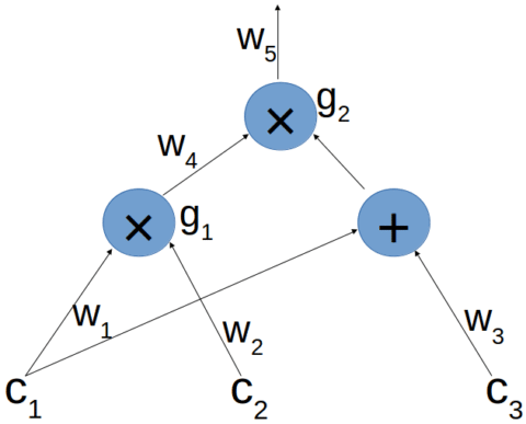
we encode the field operations as gates, each with two inputs and one output, and we refer to the edges as "wires", which line up which inputs go to which gates. There are some counterintuitive aspects of this circuit:
- wires from a single node are all labeled together as one
- we don't label addition gates
- we don't label wires from addition to multiplication gates; instead $w_1, w_3$ are both thought of as right inputs to $g_2$.
We define a legal assignment to be an assignment of values to the labeled wires, where multiplication holds. E.g. above, any $(c_1,\ldots,c_5)$ such that $c_1\cdot c_2=c_4$ and $c_5 =c_4\cdot(c_1 + c_3)$ is a legal assignment.
- Note but what about $c_1 + c_3$? These seem to be built-in to the polynomial definitions (they are sums, so as long as e.g. $R_i$ and $R_j$ are non zero, they'll get selected in the QAP below).
Back in our example, Alice can equivalently prove that she knows a legal assignment $(c_1,\ldots,c_5)$ such that $c_5 = 7$.
Reduction to QAP
For each $1, \ldots, 5$, we define $L_1,\ldots,L_5$, $R_1,\ldots,R_5$, and $O_1,\ldots,O_5$ as left wire polynomials, right wire polynomials, and output wire polynomials respectively. We then define certain constraints via selector polynomials; namely, since we have two gates $g_1, g_2$, we associate them with target points $1, 2 \in \mathbb{F}_p$ respectively, and then define constraints around the wire polynomials such that those involving gate $g_1$ output one on target point 1, zero elsewhere, and those involving gate $g_2$ output one on target point 2, zero elsewhere:
$$ L_1 = R_2 = O_4 = 2 - X $$
$$ L_4 = R_1 = R_3 = O_5 = X - 1 $$
all other polynomials are set to zero. Next define
$$ \begin{align} L &:= \sum_{i=1}^5 c_i \cdot L_i \\ R &:= \sum_{i=1}^5 c_i \cdot R_i \\ O &:= \sum_{i=1}^5 c_i \cdot O_i \\ \\ P &:= L \cdot R - O \end{align} $$
Now, we can say $(c_1, \ldots, c_5)$ is a legal assignment iff $P$ vanishes on all target points. Further, we can define a target polynomial, in this case: $T(X) = (X - 1)\cdot(X-2)$ (basically the smallest polynomial ensuring each target point is a root), and say that we have a legal assignment iff $T$ divides $P$.
A Quadratic Arithmetic Program (QAP) Q of degree $d$ and size $m$ consists of polynomials $L_1,\ldots,L_m, R_1, \ldots, R_m, O_1, \ldots, O_m$ and target polynomial $T$ of degree $d$.
An assignment $(c_1,\ldots,c_m)$ satisfies $Q$ if $L, R, O, P$ are defined as above (but to $m$ instead of 5), and $T$ divides $P$.
Bringing this back to Alice, she needs to prove she has an assignment that satisfies the $Q$ above with $c_5 = 7$.
The Pinocchio Protocol
Now we want to offer a way for Alice to prove that she knows a satisfying assignment (but let's leave off proving the final gate value for now).
Note that $T$ divides $P$ iff $P = H \cdot T$ for some polynomial $H$ of degree at most $d-2$. (Recall $T$ has degree $d$, $P = L\cdot R - O$, where $L,R, O$ have degree at most $d-1$, hence $P$ has degree at most $2d-2$, so $H$ must have degree at most $d - 2$.)
Again, Schwartz-Zippel Lemma to the rescue, if $P$ and $H \cdot T$ are different polynomials, they differ in at most $2d-2$ places. As long as $p >> 2d$, the probability that a random $s \in \mathbb{F}_p$ satisfies $P(s) = H(s) \cdot T(s)$ is negligible when these polynomials are not equal.
Protocol:
- Alice chooses $L, R, O, H$ each of degree at most $d$.
- Bob chooses random $s \in \mathbb{F}_p$ and computes $E(T(s))$.
- Note: I think Bob also sends $E(1), \ldots, E(s^d)$ to Alice for step 3.
- Alice uses blind evaluation of the polynomials evaluated at $s$: $E(L(s)), E(R(s)), E(O(s)), E(H(s))$.
- Bob uses the homomorphic properties of $E$ to check that $E(L(s) \cdot R(s) - O(s)) = E(T(s) \cdot H(s))$.
There are four more things required to turn this into a zk-SNARK:
- We need to ensure that the $L, R, O, H$ come from an actual assignment (are defined as sums with $c_i$, etc.).
- Ensure zero knowledge is learned from Alice's output.
- Under the simple group hiding $E(x) = x \cdot g$, we have only seen homomorphic addition, and haven't yet defined a way for Bob to do homomorphic multiplication (necessary in step 4 of the protocol above).
- Remove interaction from the protocol.
For (1), let $F = L + X^{d+1}\cdot R + X^{2(d+1)}\cdot O$. Now the coefficients of $L,R,O$ do not mix. Similarly for $i = 1,\ldots m$ define $F_i = L_i + X^{d+1}\cdot R_i + X^{2(d+1)}\cdot O_i$. Notice this property holds for linear combinations of the $F_i$:
$$ F_i + F_j = (L_i + L_j) + X^{d+1}\cdot (R_i + R_j) + X^{2(d+1)}\cdot(O_i + O_j).$$
If $F$ is a linear combination $\sum_{i =1}^d c_i\cdot F_i$ of these $F_i$, then because of the non-mixing of coefficients, it must also be the case that each $A = \sum_{i = 1}^d c_i \cdot A_i$ for each $A = L, R, O$. That is, the $L, R, O$ are indeed produced by an assignment $(c_1, \ldots, c_m)$.
So, Bob can have Alice prove that $F$ is a linear combination of $F_i$'s:
- Bob chooses random $\beta \in \mathbb{F}_p^{\ast}$ and sends Alice $E(\beta\cdot F_1(s)), \ldots, E(\beta\cdot F_m(s))$.
- Alice must send Bob $E(\beta\cdot F(s))$. Notice that $F(s)$ is a linear combination of the $F_i(s)$, so under the d-KCA, if she succeeds, we can assume that she does indeed know the polynomial coefficients of $F$ in terms of $F_i$.
- Note: based on the above section, I think both parties also need to send values without the $\beta$ constant.
For (2), notice we haven't introduced any randomness yet. So, for example, if Bob were to take a different assignment $(c_1', \ldots, c_m')$ and compute $L', R', O', H'$ and hidings $E(L'(s)),\ldots, E(H's))$, he can determine whether or not $(c_1,\ldots,c_m) = (c_1',\ldots,c_m')$. To avoid this, we add random $T$-shifts to each polynomial.
To be specific, Alice will choose random $\delta_1, \delta_2, \delta_3 \in \mathbb{F}_p^{\ast}$ and define
$$\begin{align*} L_z &:= L + \delta_1 \cdot T \\ R_z &:= R + \delta_2 \cdot T \\ O_z &:= O + \delta_3 \cdot T\end{align*} $$
since these are all multiples of $T$, division still holds but with a different quotient:
$$\begin{align*} L_z\cdot R_z - O_z &= (L + \delta_1 \cdot T ) \cdot (R + \delta_2 \cdot T) - (O + \delta_3 \cdot T) \\ &= L\cdot R - O + \delta_1 \cdot R \cdot T + \delta_2\cdot L \cdot T + \delta_1 \delta_2 \cdot T^2 - \delta_3 \cdot T \\ &= T \cdot (H + \delta_1 \cdot R + \delta_2 \cdot L + \delta_1\delta_2\cdot T- \delta_3) \end{align*} $$
So, defining $H_z = H + \delta_1 \cdot R + \delta_2 \cdot L + \delta_1\delta_2\cdot T- \delta_3$, we have a new set of polynomials satisfying $L_z \cdot R_z - O_z = T_z \cdot H_z$. Alice will use these instead. These polynomials mask her values: notice that $T(s)$ is nonzero with high probability (if $d << p$), so e.g. $L_z(s) = L(s) + \delta_1 \cdot T(s)$ looks like a random value now.
Pairings of Elliptic Curves
Now let's solve the last parts (3) and (4) necessary for a zk-SNARK.
To build part (3) will inevitably involve material that is not self-contained here. Recall elliptic curves from Intro to Cryptography - Chapter 6. Denote the curve $\mathcal{C}(\mathbb{F}_p)$ by $G_1$. Assume $r = |G_1|$ is prime not equal to $p$, so that any $g \ne \mathcal{O}$ generates $G_1$.
The embedding degree is the smallest integer $k$ such that $r | p^k - 1$. It is conjectured that for $k \ge 6$, the discrete log $\log(\alpha \cdot g) = \alpha$ is hard in $G_1$.
The multiplicative group of $\mathbb{F}_{p^k}$ (recall this is a group of order $\phi(p^k) = (p-1)p^{k-1}$) contains a subgroup of order $r$ that we denote $G_T$. Recall $G_1 = \mathcal{C}(\mathbb{F}p)$ and consider a larger embedding $\mathcal{C}(\mathbb{F}{p^k})$; this larger embedding contains $G_1$ and also contains another subgroup $G_2$ of order $r$ (there are actually $r$ such subgroups, but proof not shown in this article).
So to be clear, $G_T$ lives in a typical group of integers (modulo $p^k$), and $G_1,G_2$ are elliptic curves.
Fix generators $g \in G_1, h \in G_2$. There is an efficient function called the Tate reduced pairing $Tate: G_1\times G_2 \to G_T$ such that
- $Tate(g, h) = \mathbb{g}$ for a generator $\mathbb{g}$ of $G_T$.
- $Tate(a\cdot g, b \cdot h) = \mathbb{g}^{ab}$ for all $a, b \in \mathbb{F}_r$.
Now back to our setting, define
- $E_1(x) := x \cdot g,$
- $E_2(x) := x \cdot h,$
- $E(x) := x \cdot \mathbb{g},$
and note that each is homomorphic over addition, and we can compute $E(xy)$ from $E_1(x)$ and $E_2(y)$. This gives us the multiplicative "kinda homomorphism" that we need to construct, say, $E(T(s) \cdot H(s))$ from the hidings $E_1(T(s)), E_2(H(s))$.
To make this non-interactive, we'll use a (trusted-setup-style) common reference string (CRS) to start. We'll just publish Bob's first message as a CRS. So, to obtain the hiding $E(P(s))$ of Alice's polynomial $P$ at Bob's randomly chosen $s \in \mathbb{F}_r$:
Setup: Random $\alpha \in \mathbb{F}^{\ast}_r, s \in \mathbb{F}_r$ are chosen and the following CRS is published:
$$ (E_1(1), E_1(s), \ldots, E_1(s^d), \ E_2(\alpha), E_2(\alpha s), \ldots E_2(\alpha s^d)) $$
Proof: Alice computes $a = E_1(P(s))$ and $b = E_2(\alpha P(s))$ using the CRS and the same techniques above.
Verification: Bob computes and verifies equality of $Tate(a, E_2(\alpha))$ and $Tate(E_1(1), b)$:
$$ \begin{align} Tate(a, E_2(\alpha)) = Tate(P(s)\cdot g, \alpha \cdot h) &= \mathbb{g}^{\alpha P(s)} \\ &= \mathbb{g}^{1\cdot\alpha P(s)} = Tate(1\cdot g, \alpha P(s) \cdot h) = Tate(E_1(1), b) \end{align}$$
Recall under the d-KCA, Alice will only pass this verification check if $a$ is a hiding of $P(s)$ for some polynomial $P$ of degree $d$ that she knows. But in this protocol, Bob does not need to know the secret $\alpha$, since he can use the $Tate$ function to compute $E(\alpha x)$ from $E_1(x), E_2(\alpha)$.
- Note: what about the Pinocchio protocol involving $L, R, O, H$? is that involved implicitly at all in this final construction, or does that happen separately?
Bulletproof docs
TODO
Bulletproofs OG
Let $p(X) \in \mathbb{Z}p^n[X]$ be a vector polynomial $\sum{i =0}^d \textbf{p}_i \cdot X^i$. Define $q$ similarly. Let's make sure the multiplication definition makes sense:
$$ \begin{align*} p(x) = \textbf{p}0 + \textbf{p}1\cdot x + \cdots + \textbf{p}d \cdot x^d &= \begin{bmatrix} p{0,0} \\ \vdots \\ p{0, n} \end{bmatrix} + \begin{bmatrix} p{1,0} \cdot x \\ \vdots \\ p_{1, n} \cdot x \end{bmatrix} + \cdots + \begin{bmatrix} p_{d,0} \cdot x^d \\ \vdots \\ p_{d, n} \cdot x^d \end{bmatrix} \\ &= \begin{bmatrix} p_{0,0} + p_{1,0}\cdot x + \cdots + p_{d,0} \cdot x^d \\ \vdots \\ p_{0, n} + p_{1, n} \cdot x + \cdots + p_{d, n} \cdot x^d \end{bmatrix} \\ &= \begin{bmatrix} p_0(x) \\ \vdots \\ p_n(x) \end{bmatrix}\end{align*}$$
$$ \begin{align*} \langle p(x), q(x)\rangle &= \Bigg\langle \begin{bmatrix} p_{0,0} + p_{1,0}\cdot x + \cdots + p_{d,0} \cdot x^d \\ \vdots \\ p_{0, n} + p_{1, n} \cdot x + \cdots + p_{d, n} \cdot x^d \end{bmatrix} , \begin{bmatrix} q_{0,0} + q_{1,0}\cdot x + \cdots + q_{d,0} \cdot x^d \\ \vdots \\ q_{0, n} + q_{1, n} \cdot x + \cdots + q_{d, n} \cdot x^d \end{bmatrix}\Bigg\rangle \\ &= p_0(x) , q_0(x) + \cdots + p_n(x) , q_n(x) \end{align*} $$
So this is rather simple, even though the Bulletproofs paper makes a rather complicated definition. (I'm not even sure their inner product definition is correct. It looks wrong.) $p$ is just a vector whose entries are each $d$ degree polynomials over the same discriminate. An inner product between such vector polynomials is just a sum over the entry-wise polynomial multiplication. (Hadamard would similarly be defined as just entry-wise polynomial multiplication.)
ZKSummit
logUp: lookup arguments via log derivative
- Multiset equality:
- Note: sequences $(w_i)$ and $(t_j)$ are permutations of one another iff $\prod_i (X-w_i) = \prod_j (X-t_j)$ over $F$.
- Set membership: the set of $w_i$ is contained in the set of $t_j$ iff there exists $m$ such that $\prod_i (X-w_i) = \prod_j (X-t_j)^{m_j}$ over $F$
- Interopability criterion: some clever subset relation with really, really poor mathematical notation and no explanation. It has something to do with the "derivative" which is the difference between consecutive sequence elements and multiplicative factors of a lookup table.
Recall logarithmic derivative
$$ D_{log}(p(X)) = [log(p(X))]' = \frac{p'(X)}{p(X)} $$
we want this because it turns products into sums:
$$ D_{log}(p(X) \cdot q(X)) = D_{log}(p(X)) + D_{log}(q(X))$$
notice that with roots in the denominator, roots are turned into poles, with multiplicities maintained.
There is some accounting and helper functions necessary to batch these operations, but in the end you get a sum of polynomials that don't blow up in degree like they do in "PLookup".
trustlook dark pools via zk
- Current problems: large token movements create hysteria
- Dark pools keep such movements private until things settle down (like a commitment)
- Formally allowed by US under 6% GDP
- Prior work
- DeepOcean
- accountability of matchmaking service
- not compatible with decentralized markets
- Renegade.fi
- is compatible, but requires separate p2p messaging layer to operate
- NOTE this is a similar complaint to what we'd be doing with side-car IPFS
- is compatible, but requires separate p2p messaging layer to operate
- DeepOcean
teaching ZKPs
This isn't really about teaching ZKPs, this is more someone just teaching (basics of) ZKPs well. Some of the notable simplifications:
- Completeness: verifier convinced
- Soundness: prover can't cheat
- Lookup tables come into play because "looking up in memory" does not play nice with arithmetic circuits. To ensure the prover doesn't cheat, merkle trees are used.
linear algebra and zero knowledge
nice talk about generalizing common checks in terms of linear algebra equations
Short Discrete Log Proofs
An FHE ciphertext can be written as:
$$ A\vec{s} = \vec{t}$$
where $A$ is the public key, $\vec{s}$ is the message and randomness, and $\vec{t}$ is the ciphertext. The vector space is over a polynomial ring $R_q = \mathbb{Z}_q[X]/f$ for some integer $q$ and monic irreducible polynomial $f \in \mathbb{Z}[X]$ of degree $d$. This paper details a protocol for proving knowledge of $\vec{s}$, and also proving the coefficients are in the correct range. This can be combined with existing ZKPs for discrete logarithm commitments to prove arbitrary properties about $\vec{s}$.
Overall strategy
- Create a joint Pedersen commitment $t = Com(\vec{s})$ to all coefficients in $\vec{s}$.
- ZKP that
- those coefficients satisfy $A\vec{s} = \vec{t}$.
- coefficients comprise valid RWLE ciphertext
- Use existing ZKPs for discrete log commitments to prove arbitrary properties about $\vec{s}$.
Protocol overview
Setting
The first statement we prove is a simpler representation:
$$ \sum_{i = 1}^m \bm{a}_i \bm{s}_i = \bm{t} \mod (\bm{f}, q) $$
where $\bm{a}_i, \bm{s}_i, \bm{t} \in \mathcal{R}q$ and $|s{ij}| \le B$. Let $G$ be a group of size $p \le 2^{256}$ where discrete log is hard.
Step 1
The prover first rewrites this statement to move from $\mathcal{R}_q$ to $\mathbb{Z}[X]$:
$$
\sum_{i = 1}^m \bm{a}_i \bm{s}_i = \bm{t} - \bm{r}_1\cdot q - \bm{r}_2 \cdot \bm f
$$
for some polynomials $\bm r_1, \bm r_2$ that are of small degree with small coefficients.
Step 2
Prover creates Perdersen commitment $t = Com(\bm s_1, \ldots, \bm s_m, \bm r_1, \bm r_2) \in G$ where each integer coefficient of $\bm s_i, \bm r_i$ is in the exponent of a different generator $g_j$, and sends $t$ to Verifier.
Step 3
Verifier sends challenge $\alpha \in \mathbb{Z}_p$. The prover sends a proof back, consisting of:
- Range proof $\pi_{s,r}$ that proves committed values in $t$ are all in correct ranges.
- Proof that the polynomial ($\sum_{i = 1}^m \bm{a}_i \bm{s}_i = \bm{t} - \bm{r}_1\cdot q - \bm{r}_2 \cdot \bm f$) evaluated at $\alpha$ holds over $\mathbb{Z}_p$.
Note that because (1) proves the coefficients are sufficiently small, and because $q \ll p$, the polynomial evaluation in (2) should not have had any reduction modulo $p$; thus it also holds over $\mathbb{Z}[X]$, completing the proof.
We will show (2) in detail and then how to combine (1) and (2).
Step 3(a)
Define
$$
\begin{align*}
U &= [\bm a_1(\alpha) \cdots \bm a_m(\alpha) q \bm f(\alpha) ] \mod p
\\S &= \matrix{\bm s_1 }
\end{align*}
$$
TODO finish section
TODO: IPP: p16-17
TODO: main algorithm: p22
- slight deviation: instead of computing scalar multiplications at each stage, you compute a giant MSM at the end via Pippengers.
Questions
Is this related to our task of "supporting mixed bounds"?
Due to the fact that the ranges of the $\bm s_i$ and $\bm r_i$ are different, storing these in the same matrix would require us to increase the size of the matrix to accommodate the largest coefficients
- $r_i < q$, $s_i$ even smaller
- Yes!
- We want to break up $s_i$ even smaller to be more efficient
- Instead of breaking up each coefficient of $s_i$ to the same number of bits, they get broken up into different number of bits.
- 18 is largest noise for fresh ciphertext
- Stale ciphertext: probably $\alpha \cdot q / 2$, ideally power of $2$.
Is this our "gluing proofs together" task? Or is this still strictly "logproof" and we have something totally separate outside of SDLP that we glue to it?
Combining the two proofs $\pi_{r,s}$ and $\pi$ into one.
- No!
- SDLP shows: (1) and (2) on its own. It is both of these proofs.
- The "proving arbitrary properties via aforementioned very efficient ZKPs for discrete logarithm commitments" is what we're doing by gluing in bulletproofs.