EKF And Particle Filter For Localization
1.1 Motion Model Jacobian
Given state $s_t = [x_t, y_t, \theta_t]$, controls $u = [\delta_{rot1}, \delta_{trans}, \delta_{rot2}]$, we define a motion model $g(u, s_t) = s_{t+1}$ by:
$$
\begin{aligned}
& x_{t+1}=x_t+\delta_{t r a n s} * \cos \left(\theta_t+\delta_{rot1} \right) \\& y_{t+1}=y_t+\delta_{trans} * \sin \left(\theta_t+\delta_{rot1} \right) \\& \theta_{t+1}=\theta_t+\delta_{rot1}+\delta_{rot2}
\end{aligned}
$$
Derive the Jacobians of $g$ with respect to the state $G = \frac{\partial g}{\partial s_t}$ and control $V = \frac{\partial g}{\partial u}$:
$$
G=\left(\begin{array}{lll}
\frac{\partial x_{t+1}}{\partial x_t} & \frac{\partial x_{t+1}}{\partial y_t} & \frac{\partial x_{t+1}}{\partial \theta_t} \\\frac{\partial y_{t+1}}{\partial x_t} & \frac{\partial y_{t+1}}{\partial y_t} & \frac{\partial y_{t+1}}{\partial \theta_t} \\\frac{\partial \theta_{t+1}}{\partial x_t} & \frac{\partial \theta_{t+1}}{\partial y_t} & \frac{\partial \theta_{t+1}}{\partial \theta_t}
\end{array}\right) \quad V=\left(\begin{array}{ccc}
\frac{\partial x_{t+1}}{\partial \delta_{\text {rot1 }}} & \frac{\partial x_{t+1}}{\partial \delta_{\text {trans }}} & \frac{\partial x_{t+1}}{\partial \delta_{\text {rot } 2}} \\\frac{\partial y_{t+1}}{\partial \delta_{\text {rot1 }}} & \frac{\partial y_{t+1}}{\partial \delta_{\text {trans }}} & \frac{\partial y_{t+1}}{\partial \delta_{\text {rot } 2}} \\\frac{\partial \theta_{t+1}}{\partial \delta_{\text {rot1 }}} & \frac{\partial \theta_{t+1}}{\partial \delta_{\text {trans }}} & \frac{\partial \theta_{t+1}}{\partial \delta_{\text {rot } 2}}
\end{array}\right)
$$
Solution
Starting with $G$, we'll just derive this one entry at a time:
$$
\begin{align}
\frac{\partial x_{t+1}}{\partial x_t} &= \frac{\partial}{\partial x_t}x_t+\delta_{t r a n s} * \cos \left(\theta_t+\delta_{rot1} \right) &= 1 \\\frac{\partial x_{t+1}}{\partial y_t} &= \frac{\partial}{\partial y_t}x_t+\delta_{t r a n s} * \cos \left(\theta_t+\delta_{rot1} \right) &= 0 \\\frac{\partial x_{t+1}}{\partial \theta_t} &= \frac{\partial}{\partial \theta_t}x_t+\delta_{t r a n s} * \cos \left(\theta_t+\delta_{rot1} \right) &= -\delta_{trans}\sin(\theta_t + \delta_{rot1}) \\ \frac{\partial y_{t+1}}{\partial x_t} &= \frac{\partial}{\partial x_t}y_t+\delta_{trans} * \sin \left(\theta_t+\delta_{rot1} \right) &= 0 \\\frac{\partial y_{t+1}}{\partial y_t} &= \frac{\partial}{\partial y_t}y_t+\delta_{trans} * \sin \left(\theta_t+\delta_{rot1} \right) &= 1 \\\frac{\partial y_{t+1}}{\partial \theta_t} &= \frac{\partial}{\partial \theta_t}y_t+\delta_{trans} * \sin \left(\theta_t+\delta_{rot1} \right) &= \delta_{trans}\cos(\theta_t + \delta_{rot1}) \\ \frac{\partial \theta_{t+1}}{\partial x_t} &= \frac{\partial}{\partial x_t}\theta_t+\delta_{rot1}+\delta_{rot2} &= 0 \\\frac{\partial \theta_{t+1}}{\partial y_t} &= \frac{\partial}{\partial y_t}\theta_t+\delta_{rot1}+\delta_{rot2} &= 0 \\\frac{\partial \theta_{t+1}}{\partial \theta_t} &= \frac{\partial}{\partial \theta_t}\theta_t+\delta_{rot1}+\delta_{rot2} &= 1 \\\end{align}
$$
Hence
$$
G = \pmatrix{ 1 & 0 & -\delta_{trans}\sin(\theta_t + \delta_{rot1}) \\ 0 & 1 & \delta_{trans}\cos(\theta_t + \delta_{rot1}) \\ 0 & 0 & 1}
$$
Similarly for $V$:
$$
\begin{align}
\frac{\partial x_{t+1}}{\partial \delta_{rot1}} &= \frac{\partial}{\partial \delta_{rot1}}x_t+\delta_{t r a n s} * \cos \left(\theta_t+\delta_{rot1} \right) &= -\delta_{trans}\sin(\theta_t + \delta_{rot1}) \\\frac{\partial x_{t+1}}{\partial \delta_{trans}} &= \frac{\partial}{\partial \delta_{trans}}x_t+\delta_{t r a n s} * \cos \left(\theta_t+\delta_{rot1} \right) &= \cos(\theta_t + \delta_{rot1}) \\\frac{\partial x_{t+1}}{\partial \delta_{rot2}} &= \frac{\partial}{\partial \delta_{rot2}}x_t+\delta_{t r a n s} * \cos \left(\theta_t+\delta_{rot1} \right) &= 0 \\ \frac{\partial y_{t+1}}{\partial \delta_{rot1}} &= \frac{\partial}{\partial \delta_{rot1}}y_t+\delta_{trans} * \sin \left(\theta_t+\delta_{rot1} \right) &= \delta_{trans}\cos(\theta_t + \delta_{rot1}) \\\frac{\partial y_{t+1}}{\partial \delta_{trans}} &= \frac{\partial}{\partial \delta_{trans}}y_t+\delta_{trans} * \sin \left(\theta_t+\delta_{rot1} \right) &= \sin(\theta_t + \delta_{rot1}) \\\frac{\partial y_{t+1}}{\partial \delta_{rot2}} &= \frac{\partial}{\partial \delta_{rot2}}y_t+\delta_{trans} * \sin \left(\theta_t+\delta_{rot1} \right) &= 0 \\ \frac{\partial \theta_{t+1}}{\partial \delta_{rot1}} &= \frac{\partial}{\partial \delta_{rot1}}\theta_t+\delta_{rot1}+\delta_{rot2} &= 1 \\\frac{\partial \theta_{t+1}}{\partial \delta_{trans}} &= \frac{\partial}{\partial \delta_{trans}}\theta_t+\delta_{rot1}+\delta_{rot2} &= 0 \\\frac{\partial \theta_{t+1}}{\partial \delta_{rot2}} &= \frac{\partial}{\partial \delta_{rot2}}\theta_t+\delta_{rot1}+\delta_{rot2} &= 1 \\\end{align}
$$
Hence
$$
V = \pmatrix{ -\delta_{trans}\sin(\theta_t + \delta_{rot1}) & \cos(\theta_t + \delta_{rot1}) & 0 \\ \delta_{trans}\cos(\theta_t + \delta_{rot1}) & \sin(\theta_t + \delta_{rot1}) & 0 \\ 1 & 0 & 1}
$$
1.2 Observation Model Jacobian
Assume there is a landmark $l$ at position $(l_x, l_y)$.
- Suppose the robot receives measurement of the landmark in terms of the bearing angle $\phi$ relative to the direction it is currently facing. Write down the estimate for $\phi$ in terms of the landmark's position $(l_x, l_y)$ and the robot's state $(x_t, y_t, \theta_t)$.
Solution
The problem is simple when the robot is at the origin with $\theta_t = 0$. In this case $\phi = \arctan(l_y/l_x)$. But the general case can be reduced to this calculation by shifting the landmark and the robot, resulting in:
$$
\phi = \arctan\left( \frac{l_y - y_t}{l_x - x_t} \right) - \theta_t
$$
Due to the nature of $\arctan$ this formula is technically only valid when the $l_x \ge x_t$, but using $\arctan2$ should suffice in the programming assignment.
- Derive the Jacobian of the measurement with respect to the robot state:
$$
H = \pmatrix{\frac{\partial\phi}{\partial x_t} & \frac{\partial\phi}{\partial y_t} & \frac{\partial\phi}{\partial \theta_t}}
$$
Solution
$$
\begin{align}
\frac{\partial}{\partial x_t} \phi &= \frac{\partial}{\partial x_t}\arctan\left( \frac{l_y - y_t}{l_x - x_t} \right) - \theta_t \\ &= \frac{1}{1 + \left( \frac{l_y - y_t}{l_x - x_t} \right)^2} \frac{l_y - y_t}{(l_x - x_t)^2} \\&= \frac{l_y - y_t}{(l_x - x_t)^2 + (l_y - y_t)^2}
\end{align}
$$
$$
\begin{align}
\frac{\partial}{\partial y_t} \phi &= \frac{\partial}{\partial y_t}\arctan\left( \frac{l_y - y_t}{l_x - x_t} \right) - \theta_t \\ &= \frac{1}{1 + \left( \frac{l_y - y_t}{l_x - x_t} \right)^2} \frac{- 1}{l_x - x_t} \\&= \frac{x_t - l_x}{(l_x - x_t)^2 + (l_y - y_t)^2}
\end{align}
$$
$$
\begin{align}
\frac{\partial}{\partial \theta_t} \phi &= \frac{\partial}{\partial \theta_t}\arctan\left( \frac{l_y - y_t}{l_x - x_t} \right) - \theta_t \\ &= -1
\end{align}
$$
Hence
$$
H = \pmatrix{\frac{l_y - y_t}{(l_x - x_t)^2 + (l_y - y_t)^2} & \frac{x_t - l_x}{(l_x - x_t)^2 + (l_y - y_t)^2} & -1}
$$
2.1 EKF Implementation
2.1.a
2.1.b
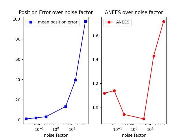
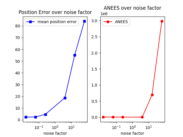
The position error increases very clearly as the noise factor increases. The ANEES (estimation error) generally increases as noise factor increases as well, but the magnitude of these errors are much lower than position error.
2.1.c
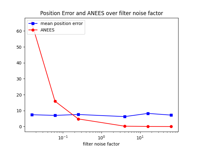
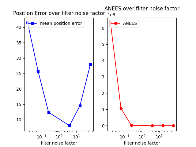
The mean position error in this graph isn't very surprising; it shows that the position error is independent of the filter noise factor, and is hence relatively constant. However, it is interesting how different the ANEES is from the initial graph. When the data factor is kept at 1, the relationship between the filter factor and ANEES is more pronounced, with a sharp dropoff as the filter factor increases.
2.1.d
The main challenge I had was reconciling the lecture slides, the tutorial, and the textbook equations to get the EKF algorithm implemented correctly. After this, I had one small hiccup with a missing minimized_angle call after the Kalman gain update that caused infrequent but large divergences between the true robot position and the estimated robot position.
2.2 PF Implementation
2.2.a
2.2.b
Similar to the EKF implementation, both position error and ANEES increase as the noise factor increases, however the the magnitude of the ANEES error is much lower than position error.
2.2.c
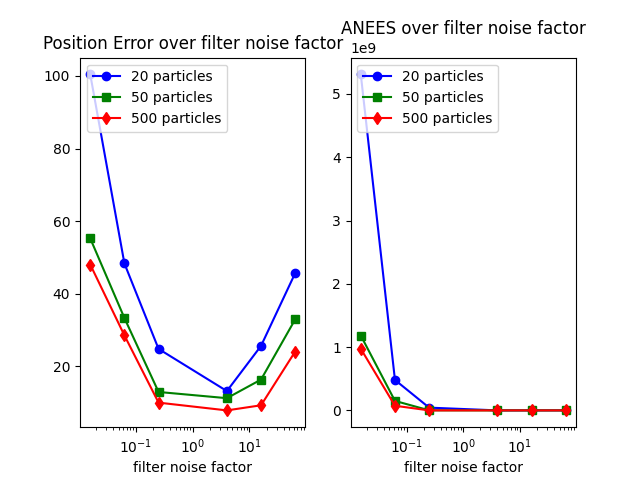
Similar to the EKF implementation, ANEES decreases as the filter noise factor increases, with a sharp dropoff. The position error seems to decrease as filter noise factor approaches 1, and then increases as filter noise factor exceeds 1.
2.2.d
These plots tell a similar story to part (c), however we get to see that, as one might expect, a larger number of particles leads to less error overall.
2.2.e
Honestly, I thought the algorithm itself was not very clearly defined across lecture, the textbook, and the starter code. The notation in the textbook is painfully ambiguous, and the textbook algorithm is described very differently than the lecture slides. For example the textbook clearly shows that the resampling happens based on weights in the current step $t$, whereas the lecture slides indicate that particles are first sampled from the previous weights at $t-1$. Discrepancies are also present in the starter code. For example in the docstring for resample:
Sample new particles and weights given current particles and weights. Be sure to use the low-variance sampler from class.
Neither the textbook nor the lecture slides indicate that weights should be sampled from a distribution, rather they should be calculated as a likelihood.
In comparison, the EKF algorithm had a very clear definition with standard linear algebra notation.
2.3 Learned Observation Model
2.3.b
I started with the tutorial code, figured how how dimensions change with maxpool options, and used a few layers with kernels and strides of dimension (2, 4) to get the last two dimensions down to 4 x 4 like the tutorial. This initial network had only 3 layers in the convolution stack. It also had three layers in the linear stack, just like the tutorial, but scaled down from 4096 to 1024 due to the lesser depth of only three convolution layers.
This didn't quite get down to 0.07 error mean, so I decided to add more convolution layers by replacing some of the (2, 4) maxpool kernels with (1, 2). This allowed the depth to reach 4096 like the tutorial, and gave me better numbers, reported below.
2.3.c
- (i)
phi:- Error Mean: 0.222006
- Error Std: 0.338984
- (ii)
xy:- Error Mean: 0.047258
- Error Std: 0.066369
- (iii) Clearly the
xysupervision mode works better thanphi. One simple explanation is that this mode uses twice the number of output channels, so the dimension doesn't need to collapse as much when outputting the final value.
2.3.d
Using the xy mode with:
python localization.py pf --use-learned-observation-model checkpoint.pt --supervision-mode xy
I observed the following five mean position errors:
7.93610.3525.34011.5346.994
2.3.e
This went fairly smoothly for me. The only challenge I had was that the initial shallow network had slightly too much error. But the very next try with a few more convolution layers worked just fine (for xy mode anyway).