Motion Planning
1.2.2 A* Implementation
(1)
| $\epsilon := 1$ | $\epsilon := 10$ | $\epsilon := 20$ | |
|---|---|---|---|
| 2dof/-o0 | cost: 78 ; states: 3003; time: 0.06 | cost: 98; states: 2177 ; time: 0.05 | cost: 106; states: 2166 ; time: 0.05 |
| 2dof/-o2 | cost: 123 ; states: 1927; time: 0.04 | cost: 165; states: 1710 ; time: 0.03 | cost: 165; states: 1710 ; time: 0.03 |
| 3dof/-o2 | cost: 168 ; states: 617585; time: 20.37 | cost: 208; states: 513023 ; time: 19.12 | cost: 208; states: 486088 ; time: 18.83 |
Obviously, as we discussed in class, as $\epsilon$ increases the solution quality is less optimal; however the running time and memory also decrease.
(2)
- 2d and 0 obstacles
- eps: 1
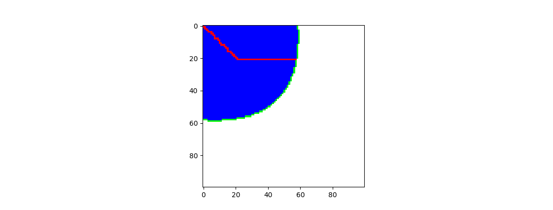
- eps: 10
- eps: 20
- eps: 1
- 2d and 1 obstacles
- eps: 1
- eps: 10
- eps: 20
- eps: 1
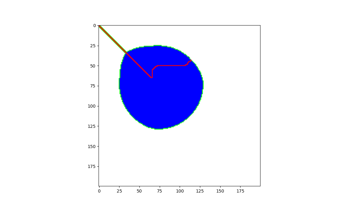
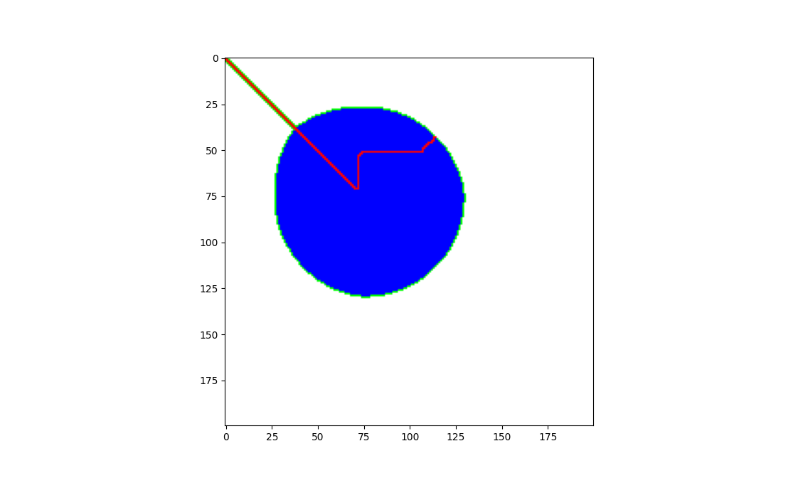
- 2d and 2 obstacles
- eps: 1
- eps: 10

- eps: 20
- eps: 1
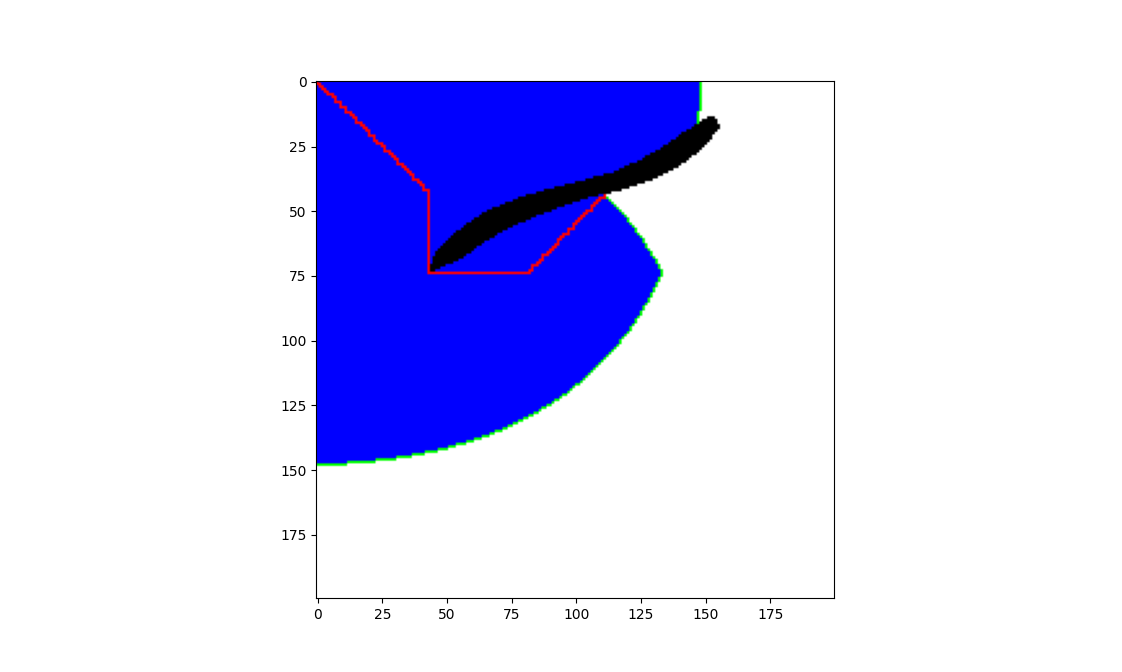
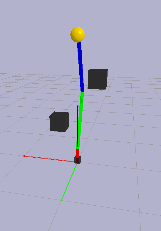
- 3d doesn't support visualization but here is a screenshot of the simulation path
(3)
If the discretization is too low fidelity, sometimes paths cannot be found. For example, running python run.py -s 3dof_robot_arm -p astar -o 2 --seed 0 with num_discretize == 10 fails to find a path. Setting discretization higher to 200 increases the cost, time, and number of states explored. Setting even higher to 500 causes the environment creation to loop for far too long (possibly forever?).
(4)
Implementing the algorithm was straightforward, but the bugs and discrepancies in the starter code versus the PDF prompt were unfortunately pretty confusing. And the structure and intent of the starter code was hard to understand. I also kept getting segmentation faults in 3d mode, until I rewrote the Astar classes.
1.2.3 RRT Implementation
(1)
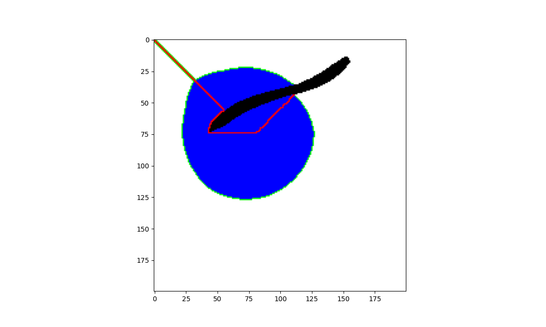
For bias of $5%$, the three scenarios resulted in the following averages:
2dof_robot_arm -o 0:- path cost: $(139.78 \pm 58.88)$
- time cost: $(0.02 \pm 0.05)$
- (generated with
./exp.sh -s 2dof_robot_arm -p rrt -o 0 -b 0.05 - figure:
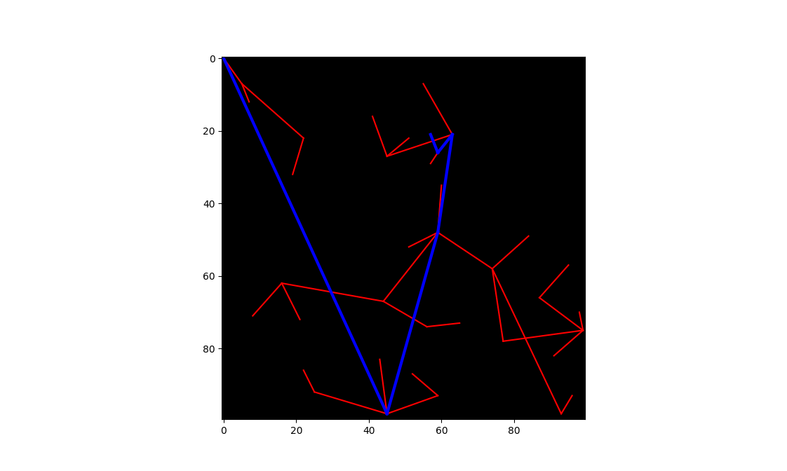
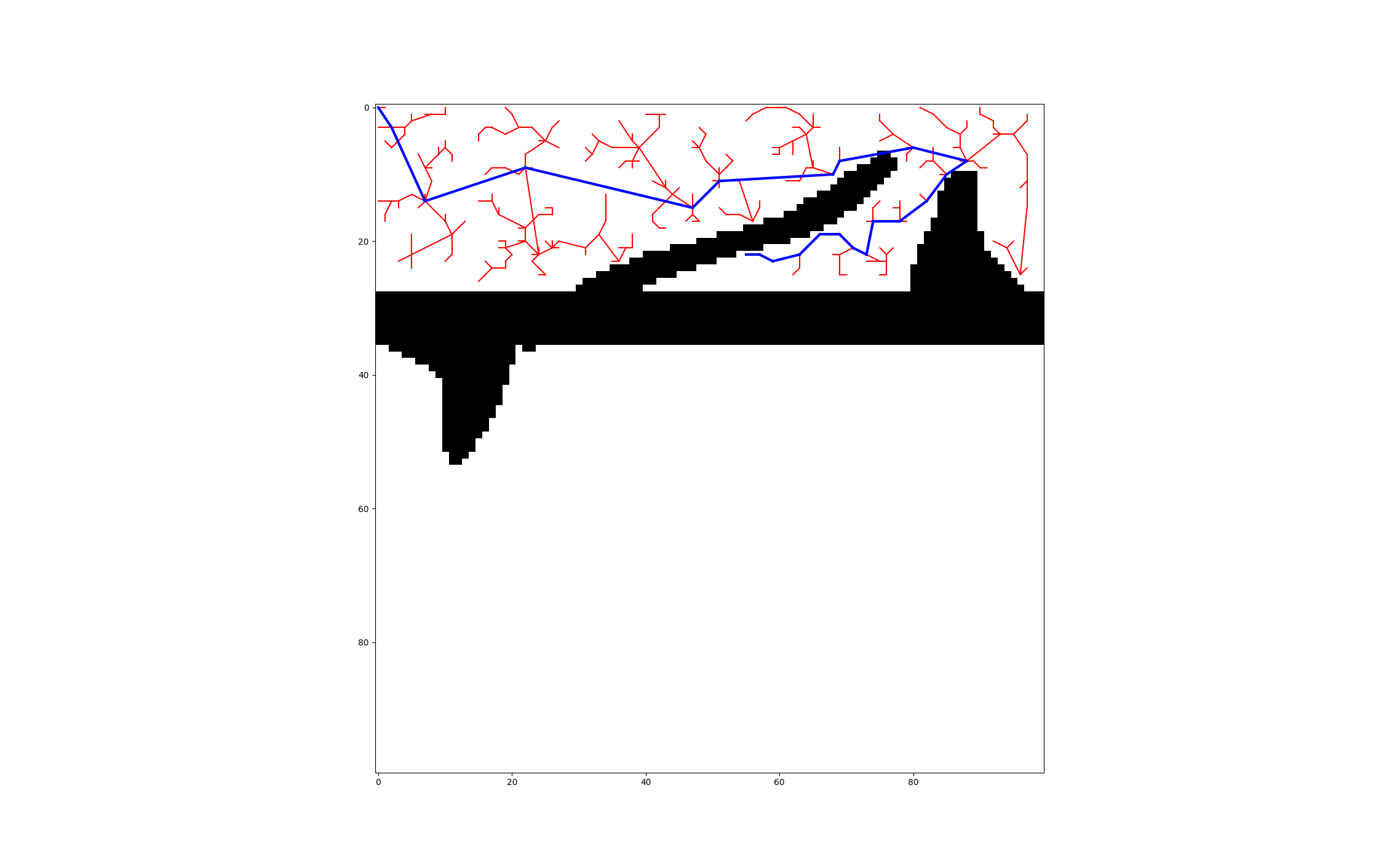
2dof_robot_arm -o 2:- path cost: $(153.87 \pm 15.28)$
- time cost: $(3.25 \pm 4.19)$
- (generated with
./exp.sh -s 2dof_robot_arm -p rrt -o 2 -b 0.05 - figure:
3dof_robot_arm -o 2:- path cost: $(198.57 \pm 84.68)$
- time cost: $(1.10 \pm 2.09)$
- (generated with
./exp.sh -s 3dof_robot_arm -p rrt -o 2 -b 0.05 - figure: not supported for 3d
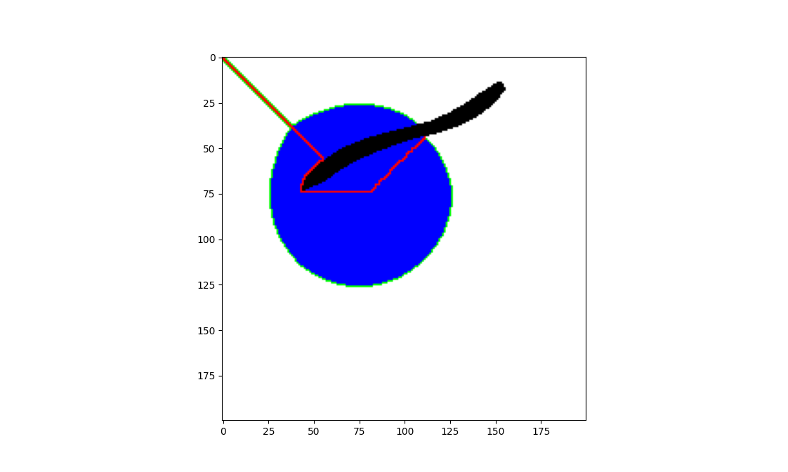
For bias of $20%$, the three scenarios resulted in the following averages:
2dof_robot_arm -o 0:- path cost: $(127.48 \pm 64.06)$
- time cost: $(0.003 \pm 0.004)$
- (generated with
./exp.sh -s 2dof_robot_arm -p rrt -o 0 -b 0.20 - figure:
2dof_robot_arm -o 2:- path cost: $(154.48 \pm 16.47)$
- time cost: $(4.49 \pm 8.50)$
- (generated with
./exp.sh -s 2dof_robot_arm -p rrt -o 2 -b 0.20 - figure:
3dof_robot_arm -o 2:- path cost: $(180.74 \pm 85.10)$
- time cost: $(0.09 \pm 0.08)$
- (generated with
./exp.sh -s 3dof_robot_arm -p rrt -o 2 -b 0.20 - figure: not supported for 3d
We can see that bias behaves like the opposite of $\epsilon$ in A*. To be specific, as bias toward the goal increases, the cost of the resulting path generally lowers to a more optimal value, however it does take more computational overhead to reach this lower cost value. This doesn't seem to always work, however, as the 2-d/2-obstacle case didn't improve.
(2)
Note that $\eta := 1$ values are all reported in part (1). Setting $\eta := 0.5$ (and keeping bias at 5%):
2dof_robot_arm -o 0:- path cost: $(97.76 \pm 24.85)$
- time cost: $(3.59 \pm 5.14)$
- (generated with
./exp.sh -s 2dof_robot_arm -p rrt -o 0 --eta 0.5) - figure:
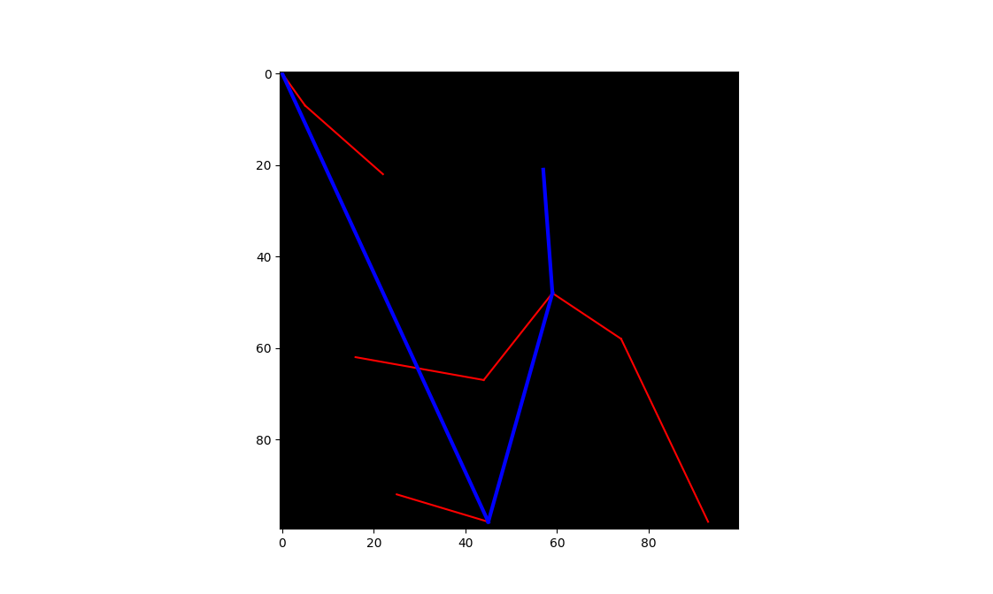
2dof_robot_arm -o 2:- path cost: $(148.41 \pm 10.57)$
- time cost: $(3.50 \pm 2.92)$
- (generated with
./exp.sh -s 2dof_robot_arm -p rrt -o 2 --eta 0.5) - figure:
3dof_robot_arm -o 2:- path cost: $(165.492 \pm 47.984)$
- time cost: $(1.608 \pm 0.523)$
- (generated with
./exp.sh -s 3dof_robot_arm -p rrt -o 2 --eta 0.5)
Note: to get $\eta = 0.5$ to work I used floating point vertices and randomized the choice of equidistant neighbors.
It seems like $\eta = 0.5$ can give you much more granular, optimal paths, but depending on the layout and number of obstacles, in some settings the increase in computational overhead would not be worth the gain in path cost optimality. So the answer is, it depends. For example, if the setting is one where a robot needs to make near-instantaneous decisions but the cost factors are not quite as important, it would make much more sense to use $\eta = 1$ rather than $\eta = 0.5$. If the robot can move slowly but distance is extremely costly (like a very big heavy robot), then $\eta = 0.5$ would make more sense.
(3)
It was exceedingly difficult to figure out the intention behind the starter code, given the lack of types. I mean, the correct return type for the path is a numpy array of tuples. That's such a strange and unconventional format. And the only way to figure this out is to hit a runtime error and try to follow the duck typing logic. In the future, if you have to use python, please include type annotations. Second, the starter code didn't pass the bias and eta values from the CLI into the planner in run.py. With a vanilla RRT/RRT* implementation there were also many spurious failures with a lower $\eta$ value, which required further modifications to the starter code and a lot of troubleshooting amongst the students. Unfortunately I spent a long, long time on this and most of it was figuring out weird idiosyncracies of the starter code, and very little was actually learning about RRT.
1.2.4 RRT* Implementation
(1)
For bias of $5%$, the three scenarios resulted in the following averages:
2dof_robot_arm -o 0:- path cost: $(68.157 \pm 6.843)$
- time cost: $(0.200 \pm 0.093)$
- (generated with
./exp.sh -s 2dof_robot_arm -p rrtstar -o 0 -b 0.05 - figure:
2dof_robot_arm -o 2:- path cost: $(117.662 \pm 3.407)$
- time cost: $(3.120 \pm 1.334)$
- (generated with
./exp.sh -s 2dof_robot_arm -p rrtstar -o 2 -b 0.05 - figure:

3dof_robot_arm -o 2:- note: fails about 20% of the time
- path cost: $(107.393 \pm 31.408)$
- time cost: $(94.672 \pm 39.143)$
- (generated with
./exp.sh -s 3dof_robot_arm -p rrtstar -o 2 -b 0.05
For bias of $20%$, the three scenarios resulted in the following averages:
2dof_robot_arm -o 0:- path cost: $(71.108 \pm 5.163)$
- time cost: $(0.234 \pm 0.084)$
- (generated with
./exp.sh -s 2dof_robot_arm -p rrtstar -o 0 -b 0.20 - figure:
2dof_robot_arm -o 2:- path cost: $(120.125 \pm 1.521)$
- time cost: $(3.202 \pm 2.027)$
- (generated with
./exp.sh -s 2dof_robot_arm -p rrtstar -o 2 -b 0.20 - figure:
3dof_robot_arm -o 2:- note: fails about 20% of the time
- path cost: $(108.813 \pm 30.153)$
- time cost: $(108.479 \pm 38.065)$
- (generated with
./exp.sh -s 3dof_robot_arm -p rrtstar -o 2 -b 0.20
Compared with RRT, it appears that bias has a much less predictable effect on RRT*. There is certainly much less of a guarantee that higher bias will reduce path cost. In fact in the examples here, the path cost tends to increase with increased bias, although this could just be noise. But it also does not seem to cost much more in time to compute.
(2)
With $\eta = 0.5$:
2dof_robot_arm -o 0:- path cost: $(69.625 \pm 9.227)$
- time cost: $(0.145 \pm 0.085)$
- (generated with
./exp.sh -s 2dof_robot_arm -p rrtstar -o 0 --eta 0.5 - figure:
2dof_robot_arm -o 2:- path cost: $(116.894 \pm 3.185)$
- time cost: $(3.157 \pm 0.988)$
- (generated with
./exp.sh -s 2dof_robot_arm -p rrtstar -o 2 --eta 0.5 - figure:
3dof_robot_arm -o 2:- path cost: $(146.216 \pm 40.822)$
- time cost: $(15.827 \pm 4.721)$
- (generated with
./exp.sh -s 3dof_robot_arm -p rrtstar -o 2 --eta 0.5
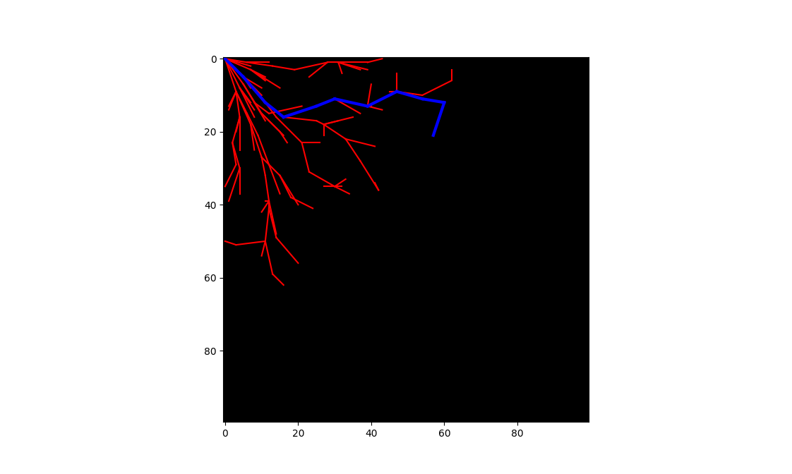
These results are interesting, and not what I expected.
- $\eta$ seems to not have much of an effect on the 2d cases
- $\eta$ clearly affects the 3d case: namely with decreased $\eta$ we see path costs increase but performance increases as well. This is in contrast with RRT, where we saw the exact opposite effect of $\eta$.
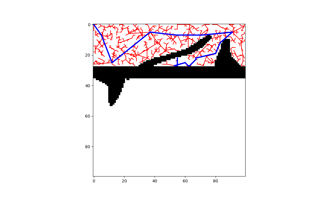
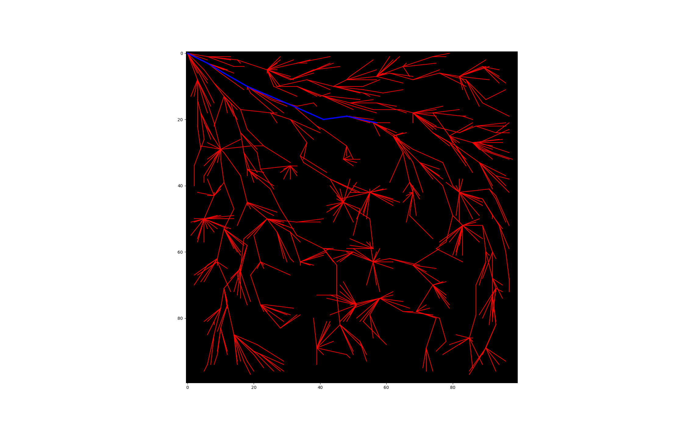
- (The graphs are also quite pretty with $\eta = 0.5$; almost reminds me of palm fronds.)
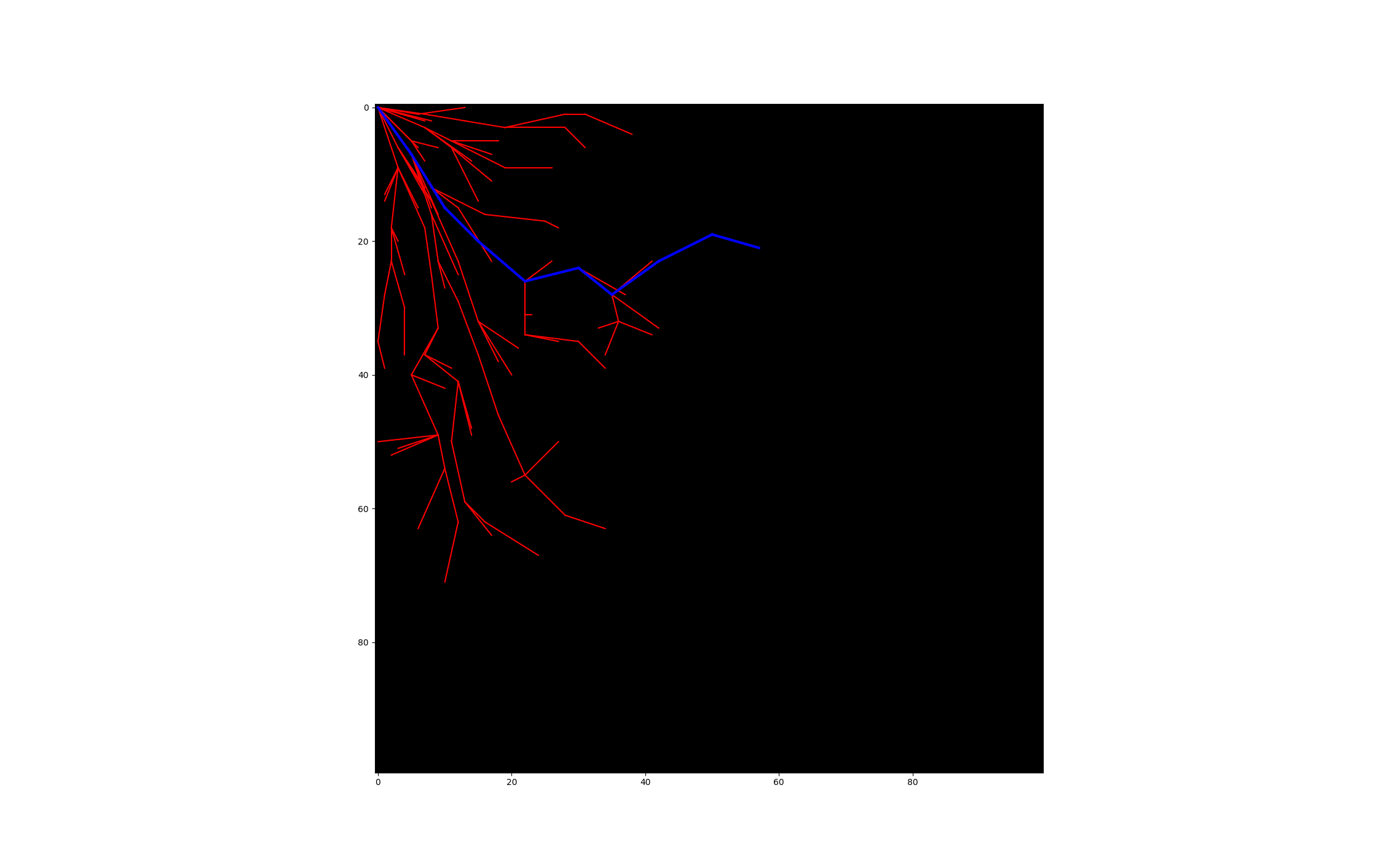
1.3.2 RRT Non-holonomic Implementation
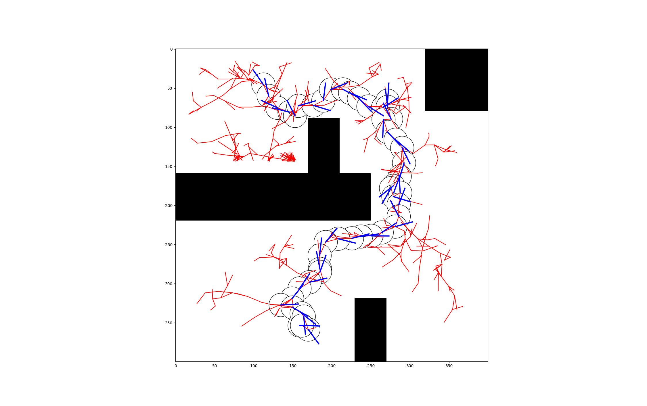
(1)
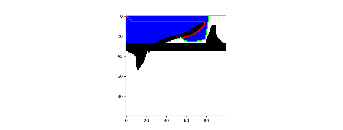
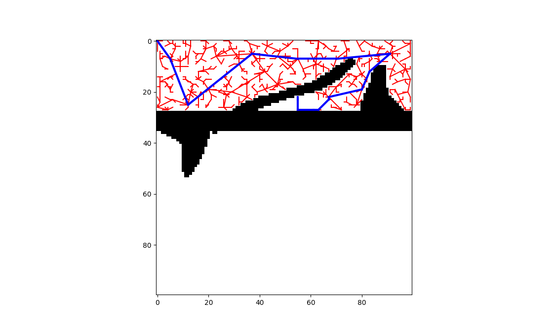
nonholrrt --bias 0.05:- path cost: $(475.000 \pm 47.129)$
- time cost: $(16.714 \pm 24.265)$
- figure:
nonholrrt --bias 0.20:- path cost: $(479.000 \pm 28.902)$
- time cost: $(14.576 \pm 11.401)$
- figure:
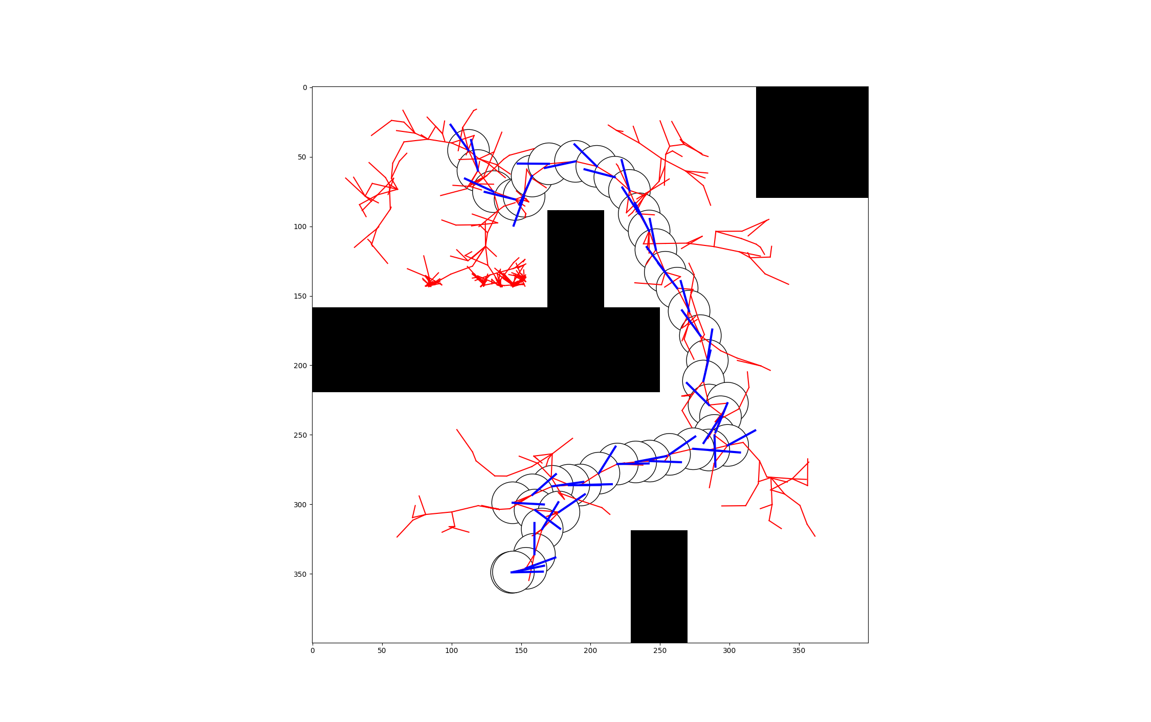
This is quite interesting in that, in most other settings, changing the bias generally resulted in tradeoffs between performance and path cost. Here, there seems to not be much of a relationship between bias and path or time costs. However, increased bias does increase the variance of the costs.
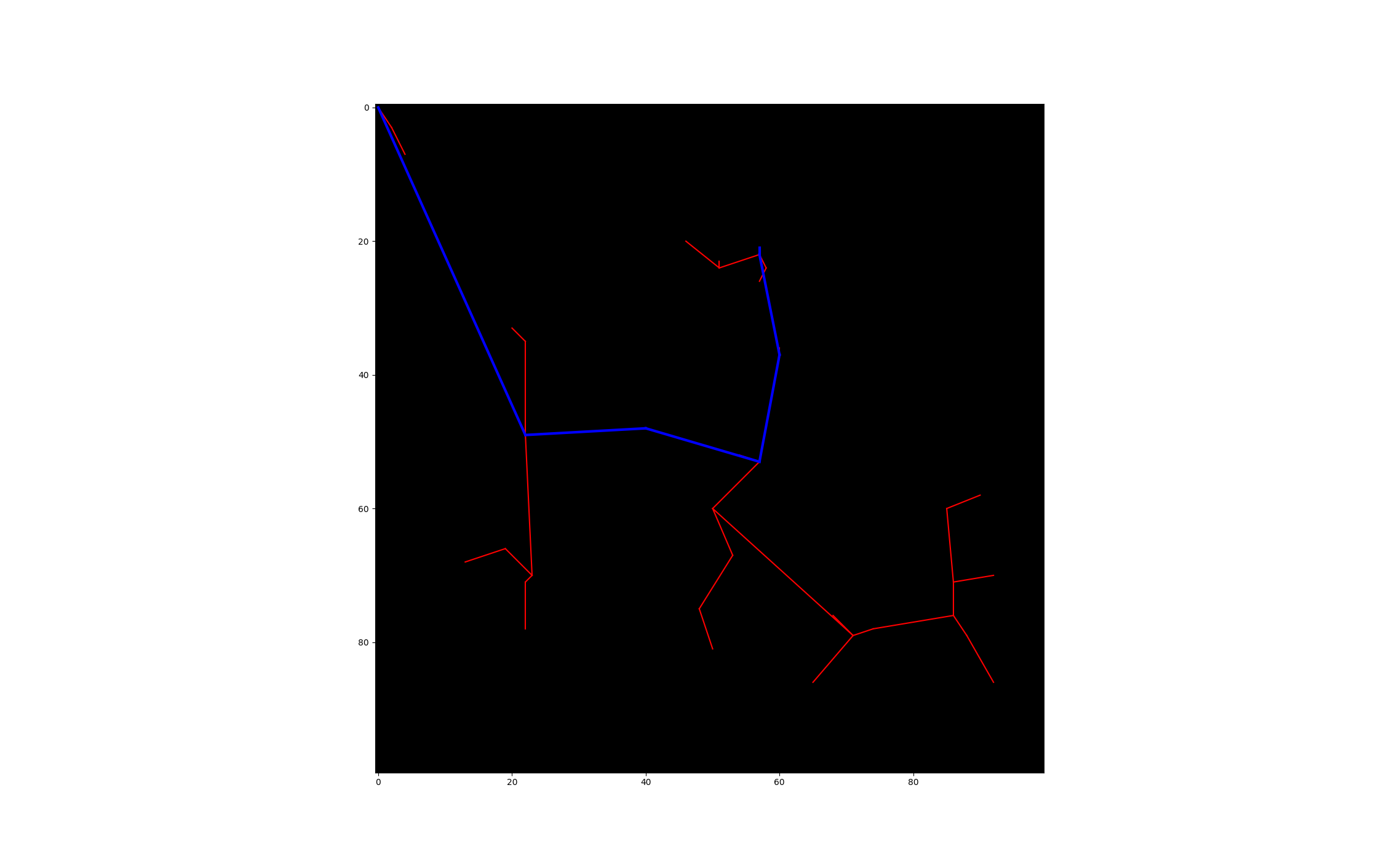
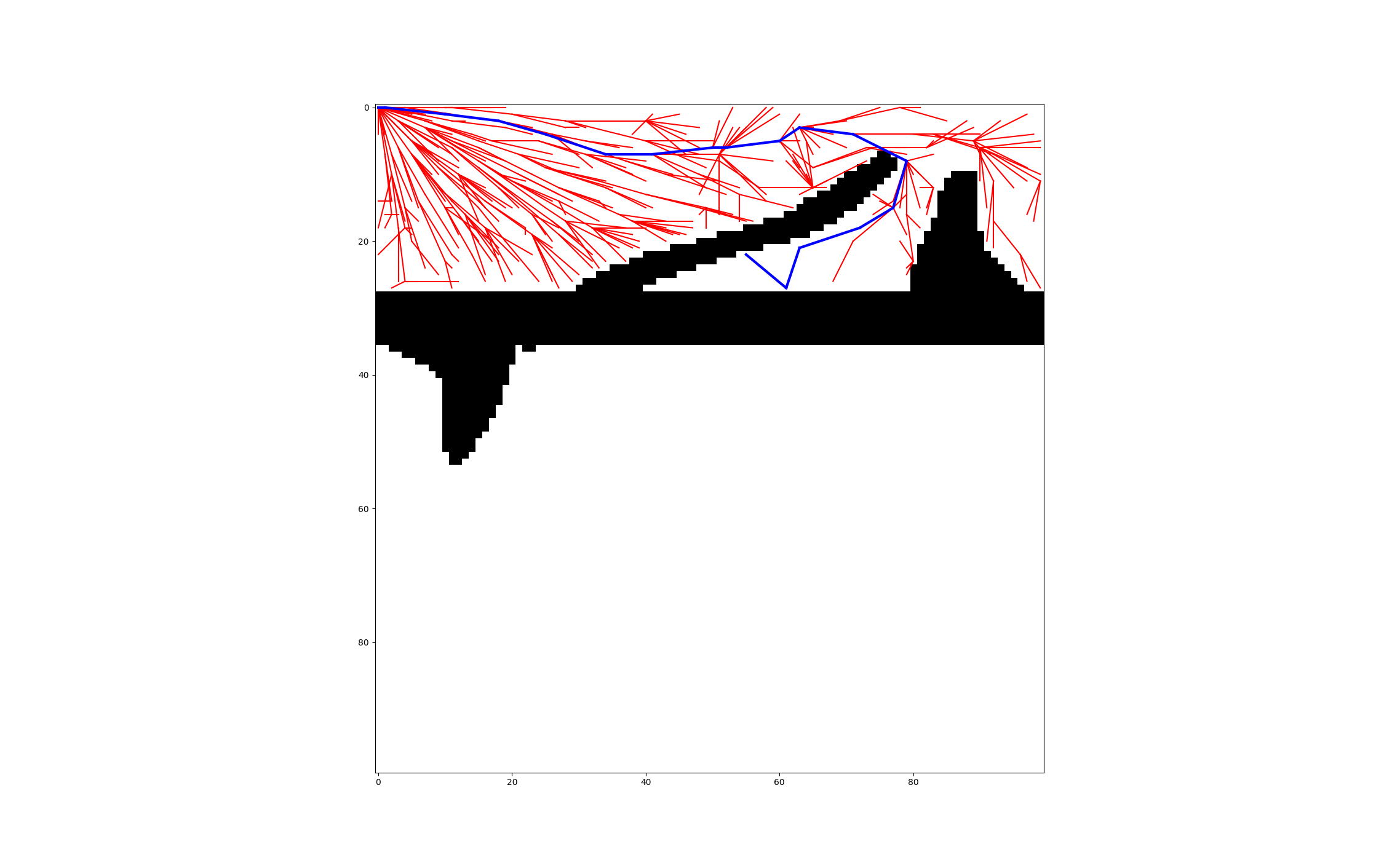
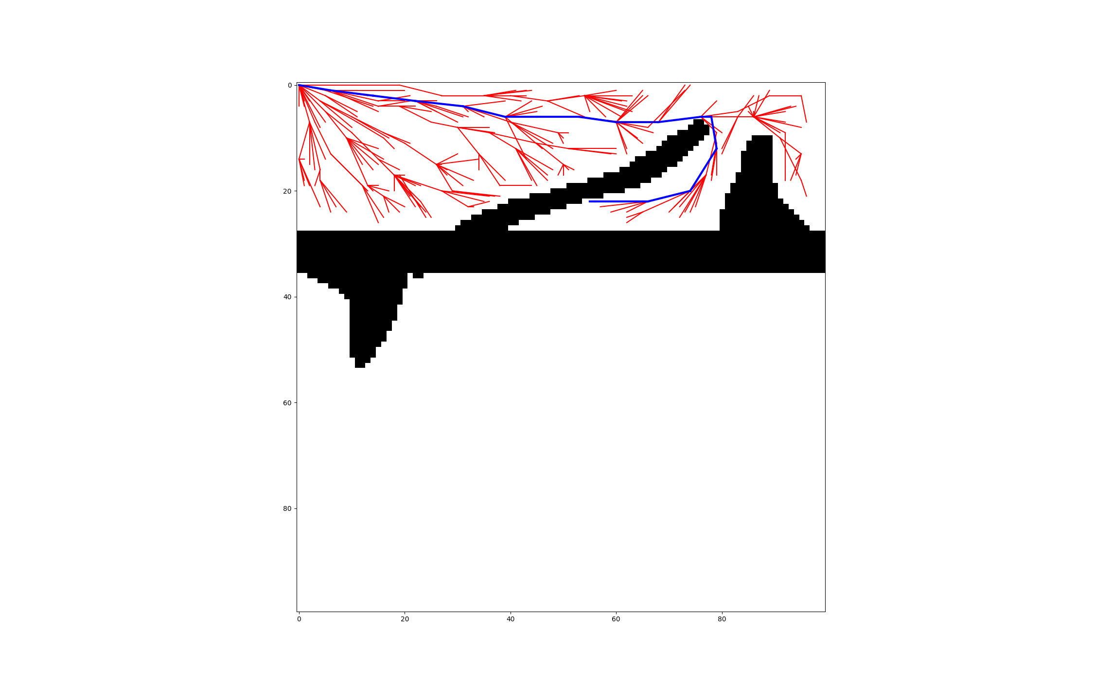
(2)
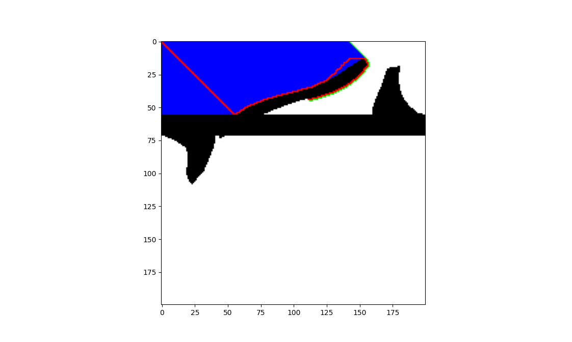
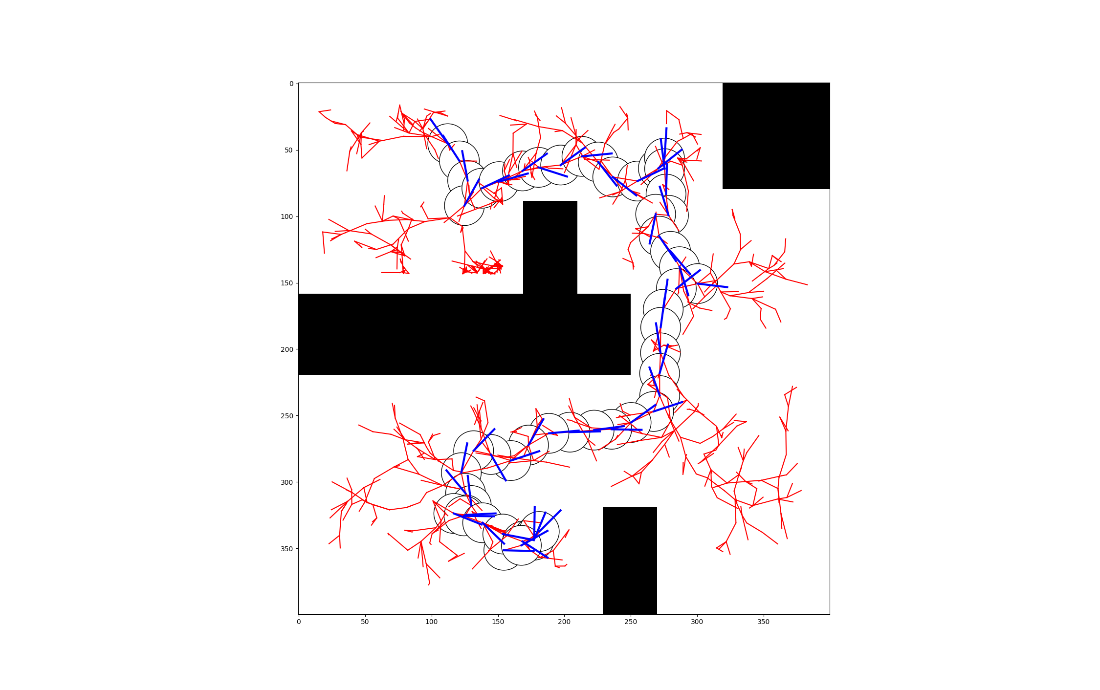
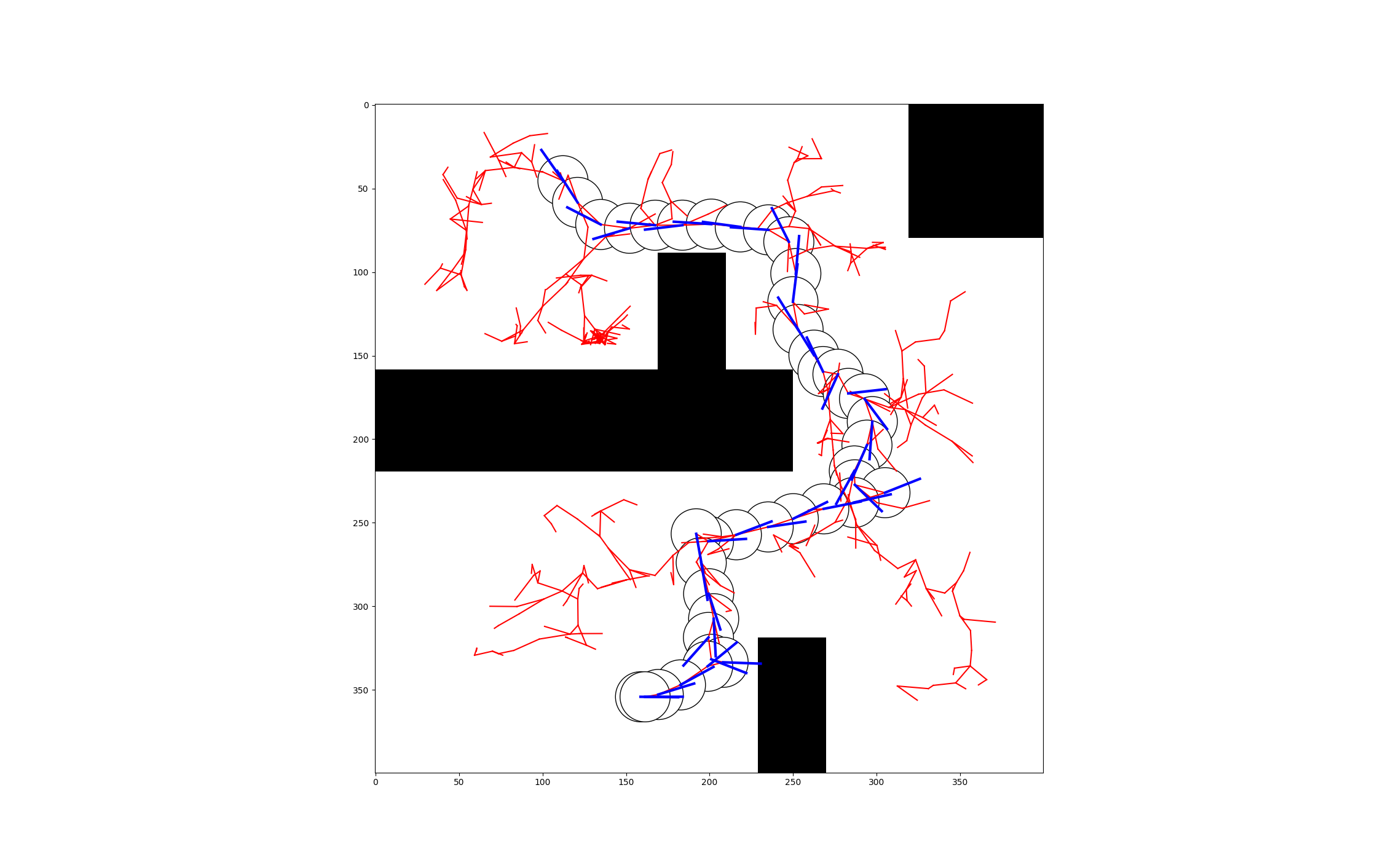
With the new distance function, time costs increase drastically, and the variability of the path cost increases. This makes sense when you look at the visualizations, as it is clear that there is much more time spent on unnecessary parts of the tree exploration. While the average path cost decreased when bias is 20%, the increased spread tells us that the cost effectiveness is inconclusive.
Note: this function is added as RRTPlannerNonholonomic.dist, but its usage is commented out in the submitted solution, so that it runs the given distance function by default.
nonholrrt --bias 0.05:- path cost: $(474.800 \pm 60.993)$
- time cost: $(46.193 \pm 79.471)$
- figure:
nonholrrt --bias 0.20:- path cost: $(462.800 \pm 65.538)$
- time cost: $(326.064 \pm 535.070)$
- figure:
(3)
This part went much more smoothly than the previous RRT/RRT* sections.